R for Data Science 1

Wickham, Hadley; Mine Çetinkaya-Rundel; & Garrett Grolemund. R for Data Science: Import, Tidy, Transform, Visualize, and Model Data. 1st Ed. O’Reilly. Home.

---

Revised

08 Jun 2023

---

Programming Environment

packages <- c(
  'hexbin',       # library(hexbin)
  'lubridate',    # library(lubridate)
  'maps',         # library(maps)
  'modelr',       # library(modelr)
  'mosaic',       # library(mosaic)
  'mosaicData',   # library(mosaicData)
  'nycflights13', # library(nycflights13)
  'pryr',         # library(pryr)
  'purrr',        # library(purrr)
  'tidyverse',    # library(tidyverse)
  'RcppRoll'      # library(RcppRoll)
)

# Install packages not yet installed
installed_packages <- packages %in% rownames(installed.packages())
if (any(installed_packages == FALSE)) {
  install.packages(packages[!installed_packages])
}

# Load packages
invisible(lapply(packages, library, character.only = TRUE))

str_c('EXECUTED : ', now())
sessionInfo()
# R.version.string # R.Version()
# .libPaths()
# installed.packages()

Attaching package: ‘lubridate’

The following objects are masked from ‘package:base’:

    date, intersect, setdiff, union

Registered S3 method overwritten by 'mosaic':
  method                           from   
  fortify.SpatialPolygonsDataFrame ggplot2

The 'mosaic' package masks several functions from core packages in order to add 
additional features.  The original behavior of these functions should not be affected by this.

Attaching package: ‘mosaic’

The following objects are masked from ‘package:dplyr’:

    count, do, tally

The following object is masked from ‘package:Matrix’:

    mean

The following object is masked from ‘package:ggplot2’:

    stat

The following object is masked from ‘package:modelr’:

    resample

The following objects are masked from ‘package:stats’:

    binom.test, cor, cor.test, cov, fivenum, IQR, median, prop.test,
    quantile, sd, t.test, var

The following objects are masked from ‘package:base’:

    max, mean, min, prod, range, sample, sum

Attaching package: ‘pryr’

The following object is masked from ‘package:mosaic’:

    inspect

The following object is masked from ‘package:dplyr’:

    where

Attaching package: ‘purrr’

The following objects are masked from ‘package:pryr’:

    compose, partial

The following object is masked from ‘package:mosaic’:

    cross

The following object is masked from ‘package:maps’:

    map

── Attaching core tidyverse packages ─────────────────────────────────────────────────────────────────────────────────────────────────────────── tidyverse 2.0.0 ──
✔ forcats 1.0.0     ✔ tibble  3.2.1
✔ readr   2.1.4     ✔ tidyr   1.3.0
✔ stringr 1.5.0     

── Conflicts ───────────────────────────────────────────────────────────────────────────────────────────────────────────────────────────── tidyverse_conflicts() ──
✖ purrr::compose()     masks pryr::compose()
✖ mosaic::count()      masks dplyr::count()
✖ purrr::cross()       masks mosaic::cross()
✖ mosaic::do()         masks dplyr::do()
✖ tidyr::expand()      masks Matrix::expand()
✖ dplyr::filter()      masks stats::filter()
✖ dplyr::lag()         masks stats::lag()
✖ purrr::map()         masks maps::map()
✖ ggformula::na.warn() masks modelr::na.warn()
✖ tidyr::pack()        masks Matrix::pack()
✖ purrr::partial()     masks pryr::partial()
✖ mosaic::resample()   masks modelr::resample()
✖ mosaic::stat()       masks ggplot2::stat()
✖ mosaic::tally()      masks dplyr::tally()
✖ tidyr::unpack()      masks Matrix::unpack()
✖ pryr::where()        masks dplyr::where()
ℹ Use the conflicted package (<http://conflicted.r-lib.org/>) to force all conflicts to become errors

'EXECUTED : 2024-06-20 10:49:11.689784'

R version 4.3.0 (2023-04-21)
Platform: aarch64-apple-darwin20 (64-bit)
Running under: macOS 14.5

Matrix products: default
BLAS:   /Library/Frameworks/R.framework/Versions/4.3-arm64/Resources/lib/libRblas.0.dylib 
LAPACK: /Library/Frameworks/R.framework/Versions/4.3-arm64/Resources/lib/libRlapack.dylib;  LAPACK version 3.11.0

locale:
[1] en_US.UTF-8/en_US.UTF-8/en_US.UTF-8/C/en_US.UTF-8/en_US.UTF-8

time zone: America/New_York
tzcode source: internal

attached base packages:
[1] stats     graphics  grDevices utils     datasets  methods   base     

other attached packages:
 [1] RcppRoll_0.3.0     forcats_1.0.0      stringr_1.5.0      readr_2.1.4       
 [5] tidyr_1.3.0        tibble_3.2.1       tidyverse_2.0.0    purrr_1.0.2       
 [9] pryr_0.1.6         nycflights13_1.0.2 mosaic_1.8.4.2     mosaicData_0.20.3 
[13] ggformula_0.10.4   dplyr_1.1.2        Matrix_1.5-4       ggplot2_3.4.3     
[17] lattice_0.21-8     modelr_0.1.11      maps_3.4.1         lubridate_1.9.2   
[21] hexbin_1.28.3     

loaded via a namespace (and not attached):
 [1] utf8_1.2.3         generics_0.1.3     stringi_1.7.12     hms_1.1.3         
 [5] digest_0.6.31      magrittr_2.0.3     evaluate_0.21      grid_4.3.0        
 [9] timechange_0.2.0   pbdZMQ_0.3-9       fastmap_1.1.1      jsonlite_1.8.5    
[13] backports_1.4.1    fansi_1.0.4        scales_1.2.1       tweenr_2.0.2      
[17] codetools_0.2-19   cli_3.6.1          labelled_2.11.0    rlang_1.1.1       
[21] crayon_1.5.2       polyclip_1.10-4    munsell_0.5.0      base64enc_0.1-3   
[25] withr_2.5.0        repr_1.1.6         tools_4.3.0        tzdb_0.4.0        
[29] uuid_1.1-0         colorspace_2.1-0   mosaicCore_0.9.2.1 broom_1.0.5       
[33] IRdisplay_1.1      vctrs_0.6.3        R6_2.5.1           ggridges_0.5.4    
[37] lifecycle_1.0.3    ggstance_0.3.6     MASS_7.3-58.4      pkgconfig_2.0.3   
[41] pillar_1.9.0       gtable_0.3.3       glue_1.6.2         Rcpp_1.0.10       
[45] ggforce_0.4.1      haven_2.5.2        tidyselect_1.2.0   IRkernel_1.3.2    
[49] farver_2.1.1       htmltools_0.5.5    compiler_4.3.0    

---

03 - Data Visualization

head(x = mpg, n = 5)

A tibble: 5 × 11

manufacturer	model	displ	year	cyl	trans	drv	cty	hwy	fl	class
<chr>	<chr>	<dbl>	<int>	<int>	<chr>	<chr>	<int>	<int>	<chr>	<chr>
audi	a4	1.8	1999	4	auto(l5)	f	18	29	p	compact
audi	a4	1.8	1999	4	manual(m5)	f	21	29	p	compact
audi	a4	2.0	2008	4	manual(m6)	f	20	31	p	compact
audi	a4	2.0	2008	4	auto(av)	f	21	30	p	compact
audi	a4	2.8	1999	6	auto(l5)	f	16	26	p	compact

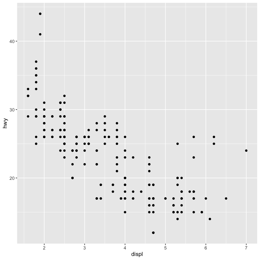
ggplot(data=mpg) +
  geom_point(mapping=aes(x=displ,y=hwy))
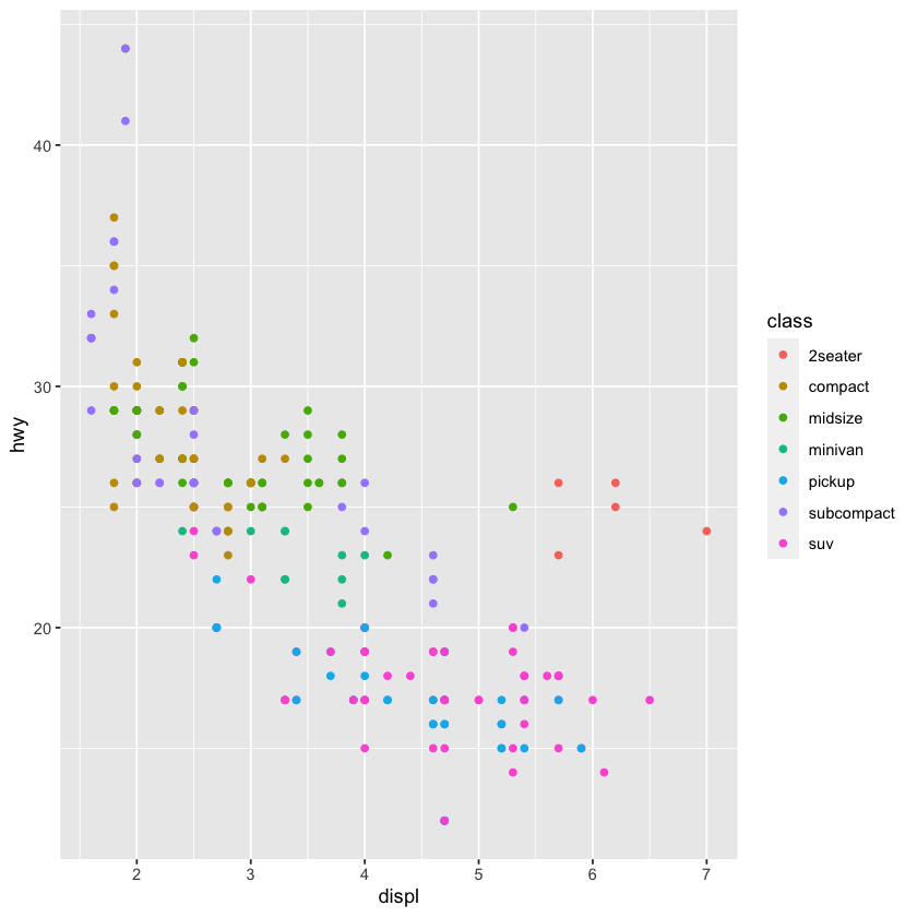
ggplot(data=mpg) +
  geom_point(mapping=aes(x=displ,y=hwy,color=class))
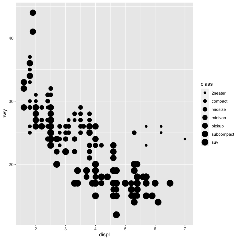
ggplot(data=mpg) +
  geom_point(mapping=aes(x=displ,y=hwy,size=class))
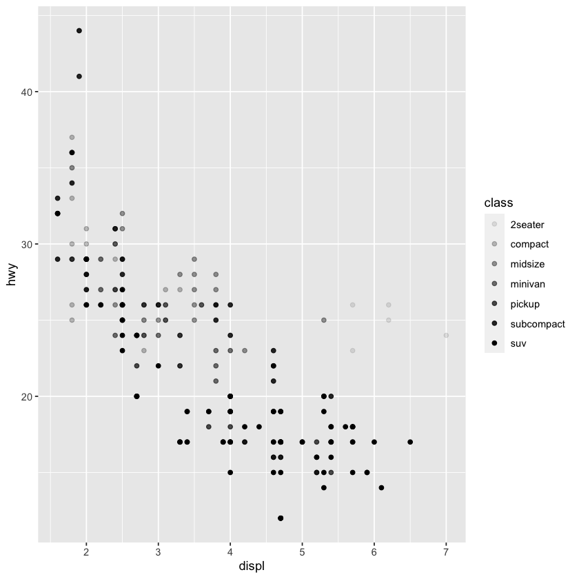
ggplot(data=mpg) +
  geom_point(mapping=aes(x=displ,y=hwy,alpha=class))
ggplot(data=mpg) +
  geom_point(mapping=aes(x=displ,y=hwy,shape=class))

Warning message:
“Using size for a discrete variable is not advised.”

Warning message:
“Using alpha for a discrete variable is not advised.”

Warning message:
“The shape palette can deal with a maximum of 6 discrete values because
more than 6 becomes difficult to discriminate; you have 7. Consider
specifying shapes manually if you must have them.”

Warning message:
“Removed 62 rows containing missing values (`geom_point()`).”

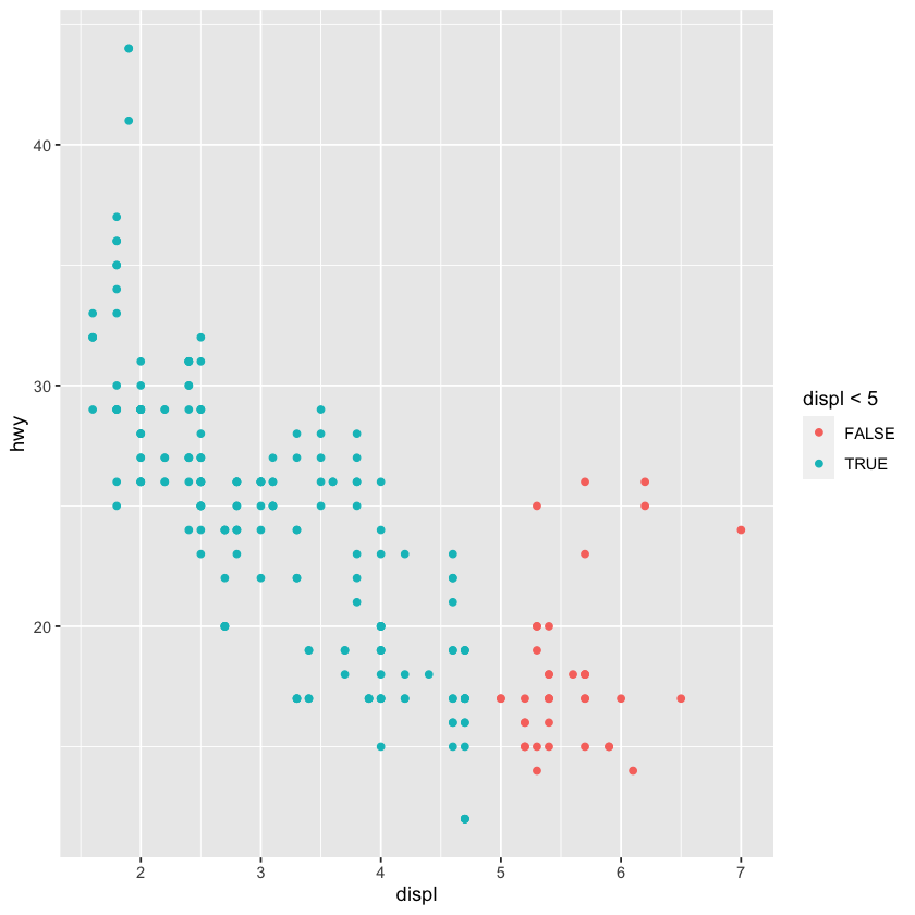
ggplot2::mpg %>%
  ggplot() +
    geom_point(mapping=aes(x=displ, y=hwy, color=displ<5))

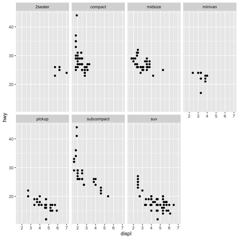
ggplot2::mpg %>%
  ggplot() +
    geom_point(mapping = aes(x = displ, y = hwy)) +
    facet_wrap(~ class, nrow=2)
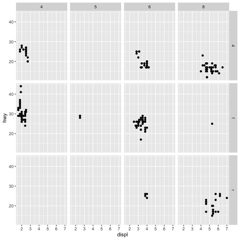
ggplot2::mpg %>%
  ggplot() +
    geom_point(mapping = aes(x = displ, y = hwy)) +
    facet_grid(drv ~ cyl)

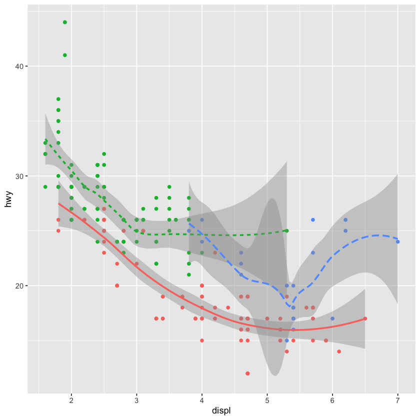
ggplot2::mpg %>%
  ggplot(mapping = aes(x = displ, y = hwy, color = drv)) +
    geom_point (                               show.legend=FALSE) +
    geom_smooth(mapping = aes(linetype = drv), show.legend=FALSE)

`geom_smooth()` using method = 'loess' and formula = 'y ~ x'

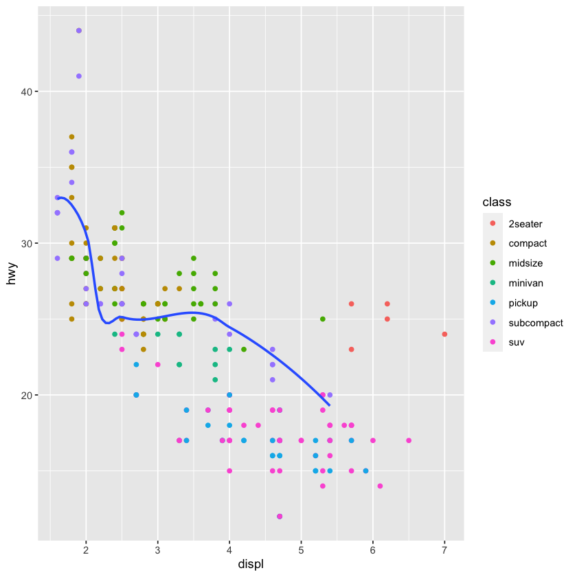
ggplot2::mpg %>%
  ggplot(mapping = aes(x = displ, y = hwy)) +
    geom_point(mapping = aes(color = class)) +
    geom_smooth(data = filter(mpg, class == 'subcompact'), se=FALSE)

`geom_smooth()` using method = 'loess' and formula = 'y ~ x'

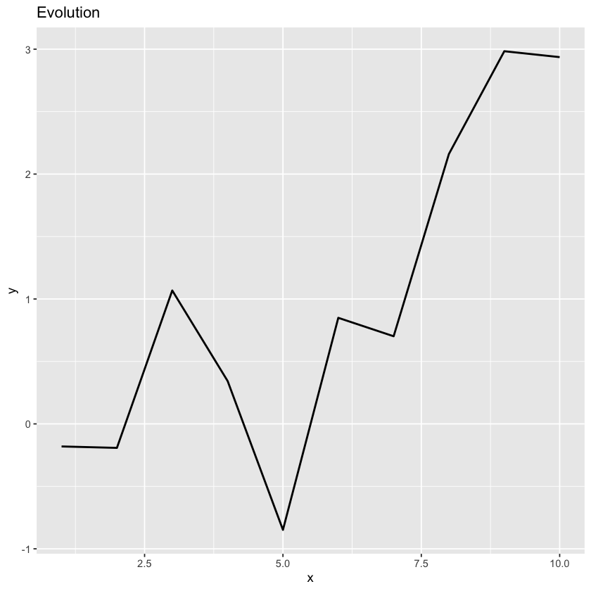
# LINE PLOT
x  <- 1:10
y  <- cumsum(rnorm(10))
df <- data.frame(x, y)
ggplot(df, mapping = aes(x = x, y = y)) +
  geom_line(size=0.8) +
  ggtitle('Evolution')

Warning message:
“Using `size` aesthetic for lines was deprecated in ggplot2 3.4.0.
ℹ Please use `linewidth` instead.”

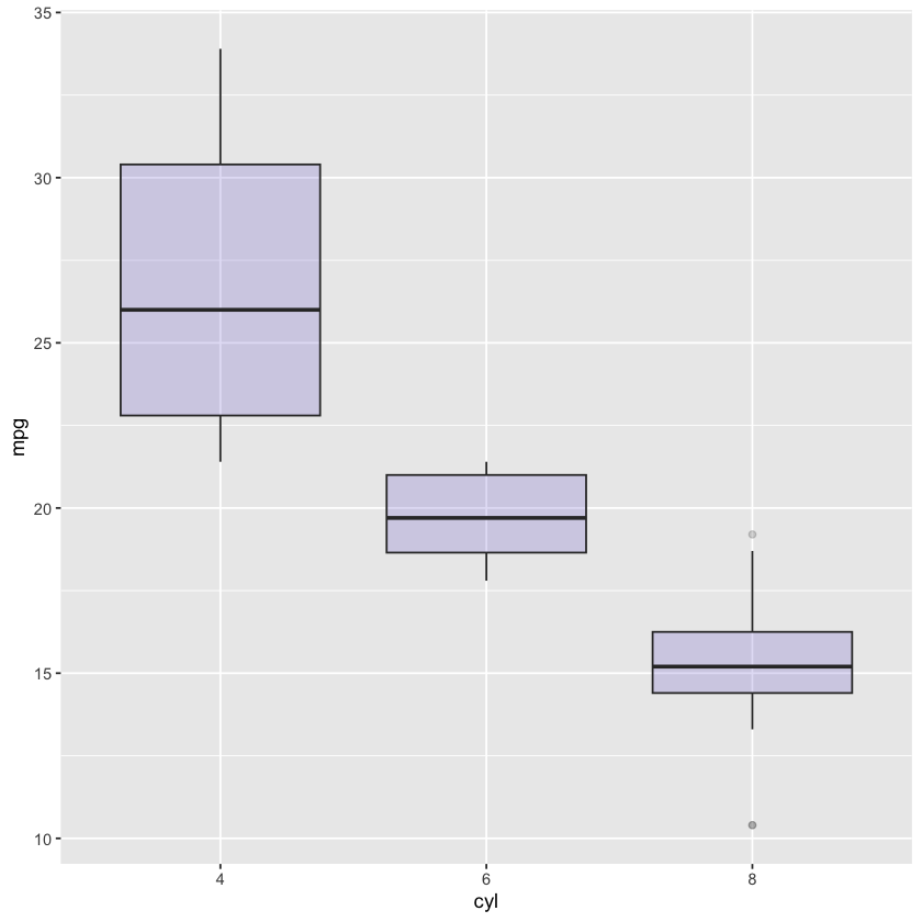
# BOX PLOT
mtcars %>%
  ggplot(mapping = aes(x = as.factor(cyl), y = mpg)) +
    geom_boxplot(fill = 'slateblue', alpha = 0.2) +
    xlab('cyl')

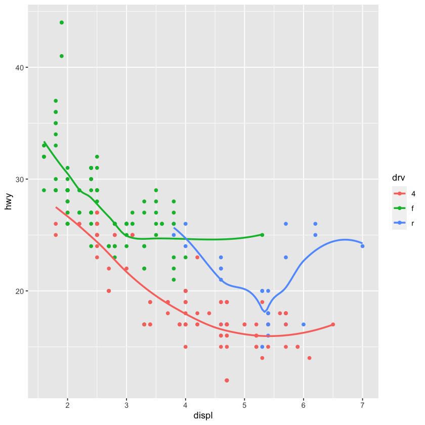
ggplot(data    = mpg,
       mapping = aes(x     = displ,
                     y     = hwy,
                     color = drv)) +
  geom_point() +
  geom_smooth(se=FALSE)

`geom_smooth()` using method = 'loess' and formula = 'y ~ x'

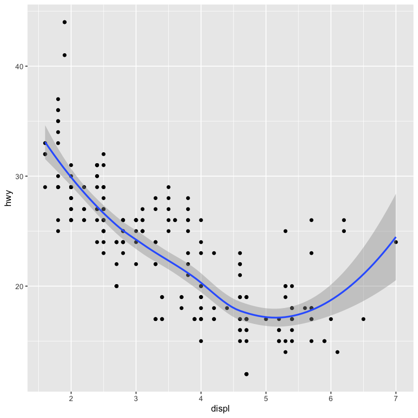
ggplot(data    = mpg,
       mapping = aes(x = displ,
                     y = hwy)) +
  geom_point () +
  geom_smooth()

ggplot() +
  geom_point (data    = mpg,
              mapping = aes(x = displ,
                            y = hwy)) +
  geom_smooth(data    = mpg,
              mapping = aes(x = displ,
                            y = hwy))

`geom_smooth()` using method = 'loess' and formula = 'y ~ x'

`geom_smooth()` using method = 'loess' and formula = 'y ~ x'

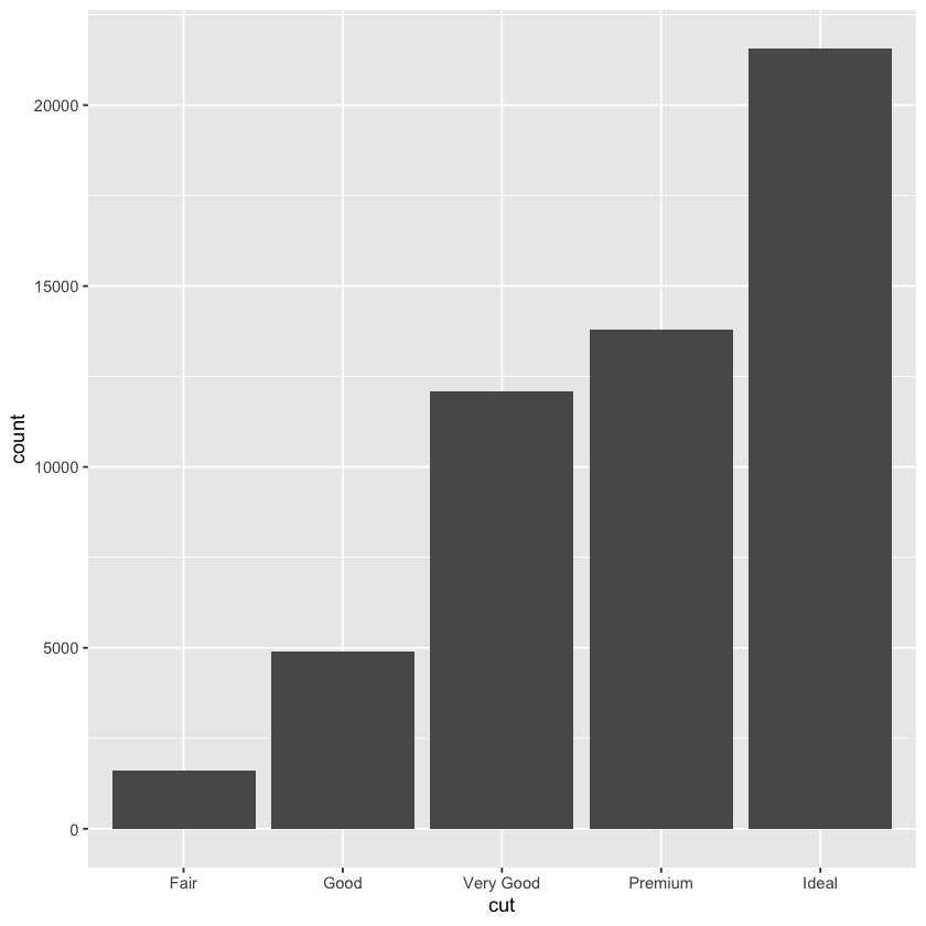
ggplot(data = diamonds) +
  geom_bar  (mapping = aes(x = cut))
ggplot(data = diamonds) +
  stat_count(mapping = aes(x = cut))

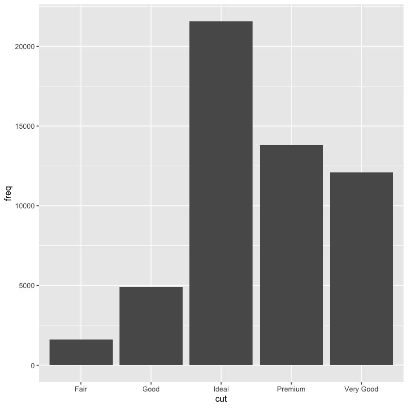
demo <- tribble(
  ~cut,  ~freq,
  'Fair',      1610,
  'Good',      4906,
  'Very Good',12082,
  'Premium',  13791,
  'Ideal',    21551
)
ggplot(data = demo) +
  geom_bar(mapping = aes(x = cut,
                         y = freq),
           stat    = 'identity')

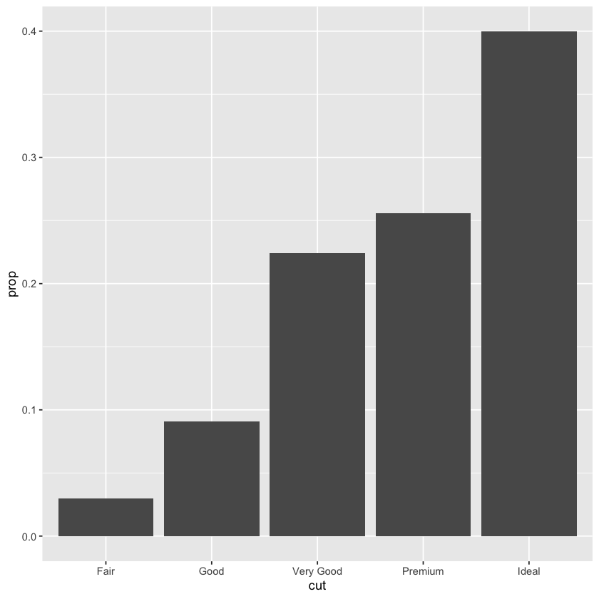
ggplot(data = diamonds) +
  geom_bar(mapping = aes(x     = cut,
                         y     = stat(prop),
                         group = 1))

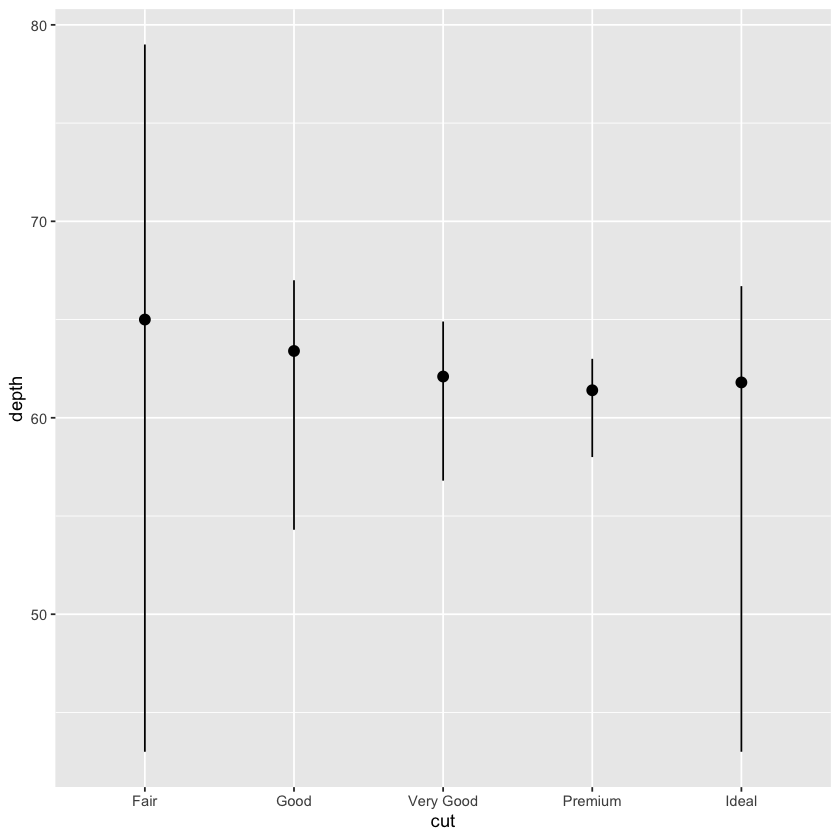
ggplot(data = diamonds) +
  stat_summary(
    mapping = aes(x = cut, y = depth),
    fun.min = min,
    fun.max = max,
    fun     = median
  )
ggplot(data = diamonds) +
  geom_pointrange(
    mapping = aes(x = cut, y = depth),
    stat    = 'summary',
    fun.min = min,
    fun.max = max,
    fun     = median
  )

Warning message:
“`stat(prop)` was deprecated in ggplot2 3.4.0.
ℹ Please use `after_stat(prop)` instead.”

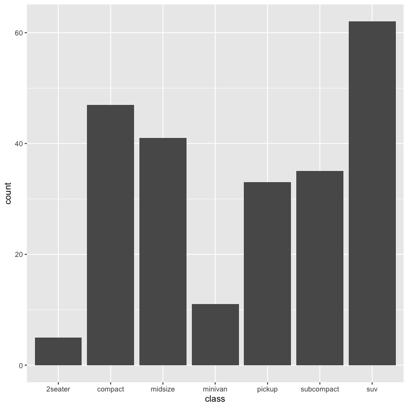
g  <- ggplot(data = mpg, mapping = aes(x = class))

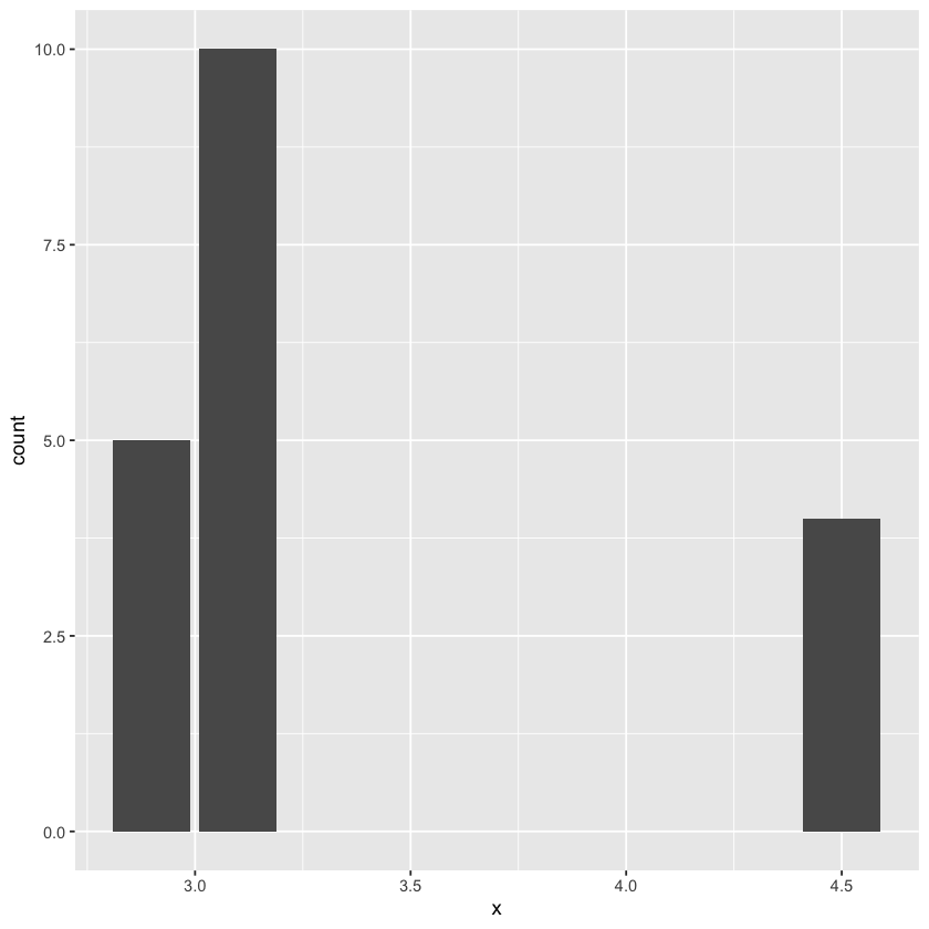
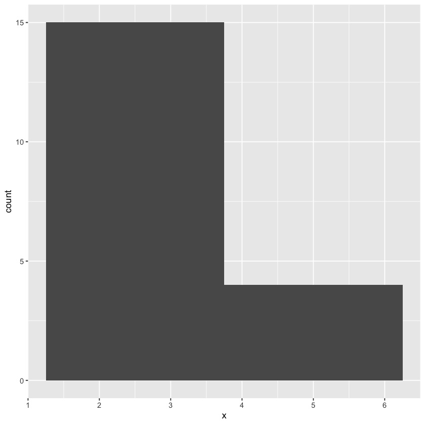
df <- data.frame(x = rep(c(2.9, 3.1, 4.5), c(5, 10, 4)))
ggplot(data = df, mapping = aes(x)) + geom_bar()
ggplot(data = df, mapping = aes(x)) + geom_histogram(binwidth = 2.5)
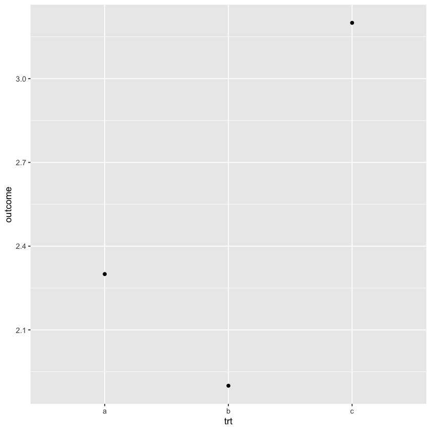
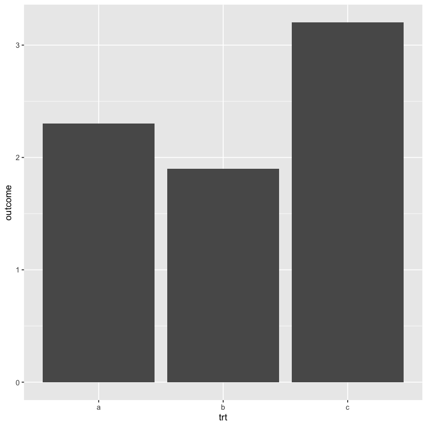
df <- data.frame(trt = c('a', 'b', 'c'), outcome = c(2.3, 1.9, 3.2))
ggplot(data = df,  mapping = aes(x = trt, y = outcome)) + geom_point()
ggplot(data = df,  mapping = aes(x = trt, y = outcome)) + geom_col()
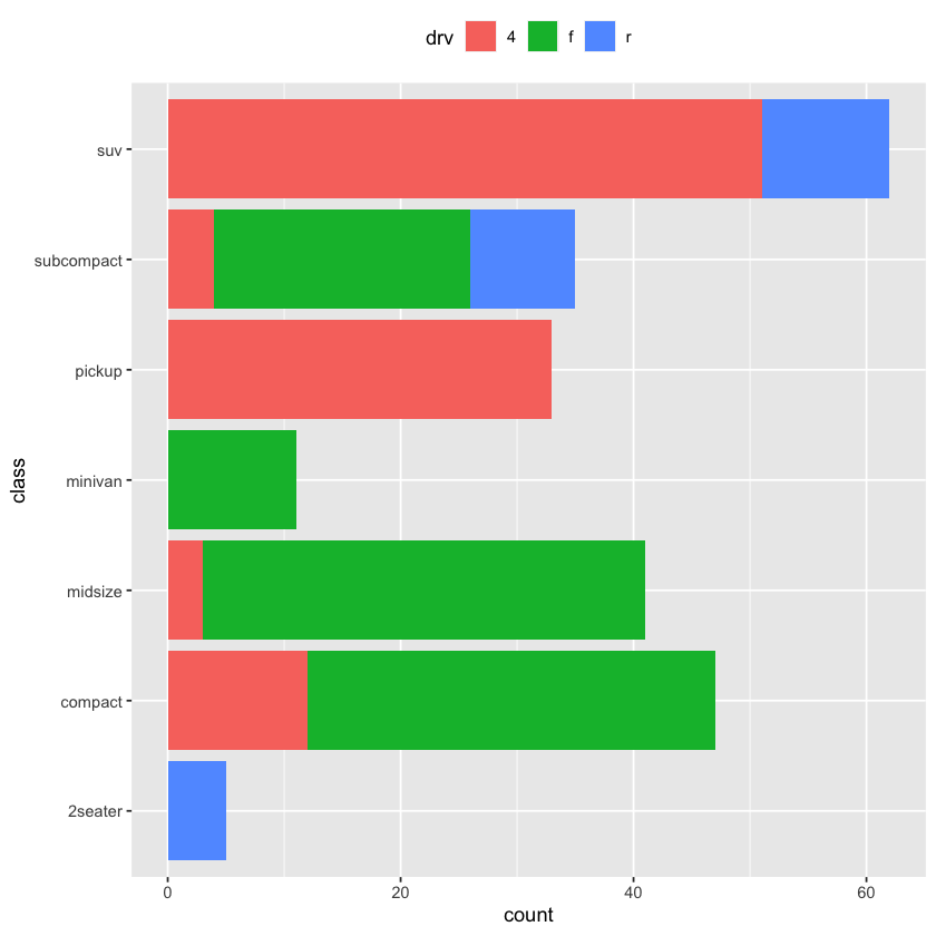
ggplot(data = mpg, mapping = aes(y = class)) + geom_bar(mapping = aes(fill = drv), position = position_stack(reverse = TRUE)) + theme(legend.position='top')
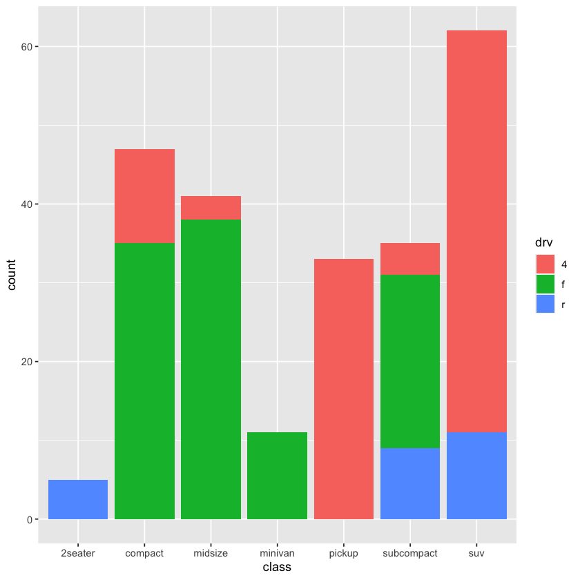
g + geom_bar(mapping = aes(fill = drv))
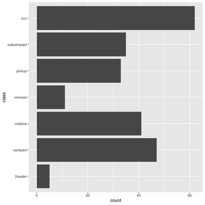
ggplot(data = mpg, mapping = aes(y = class)) + geom_bar()
g + geom_bar(mapping = aes(weight = displ))
g + geom_bar()

# 3.7.1 [5]

ggplot(data = diamonds) +
  geom_bar(mapping = aes(x = cut, y = after_stat(prop), group = 1))
ggplot(data = diamonds) +
  geom_bar(mapping = aes(x = cut, y = after_stat(prop), fill = color))

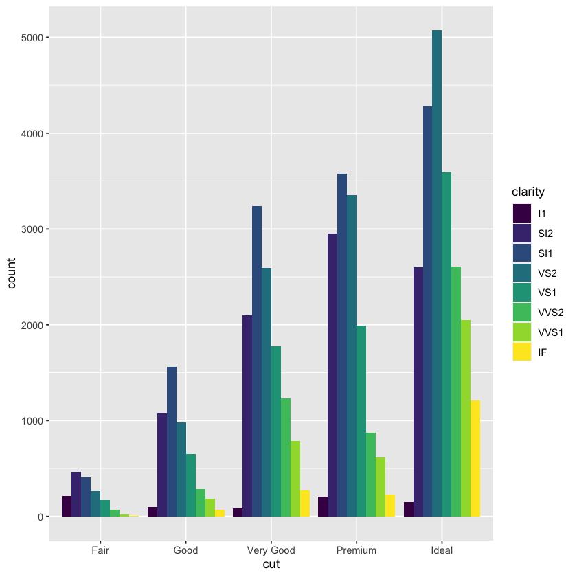
ggplot(data = diamonds) +
  geom_bar(mapping = aes(x = cut, fill = clarity), position = 'dodge')
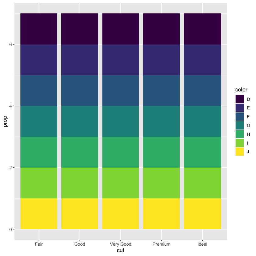
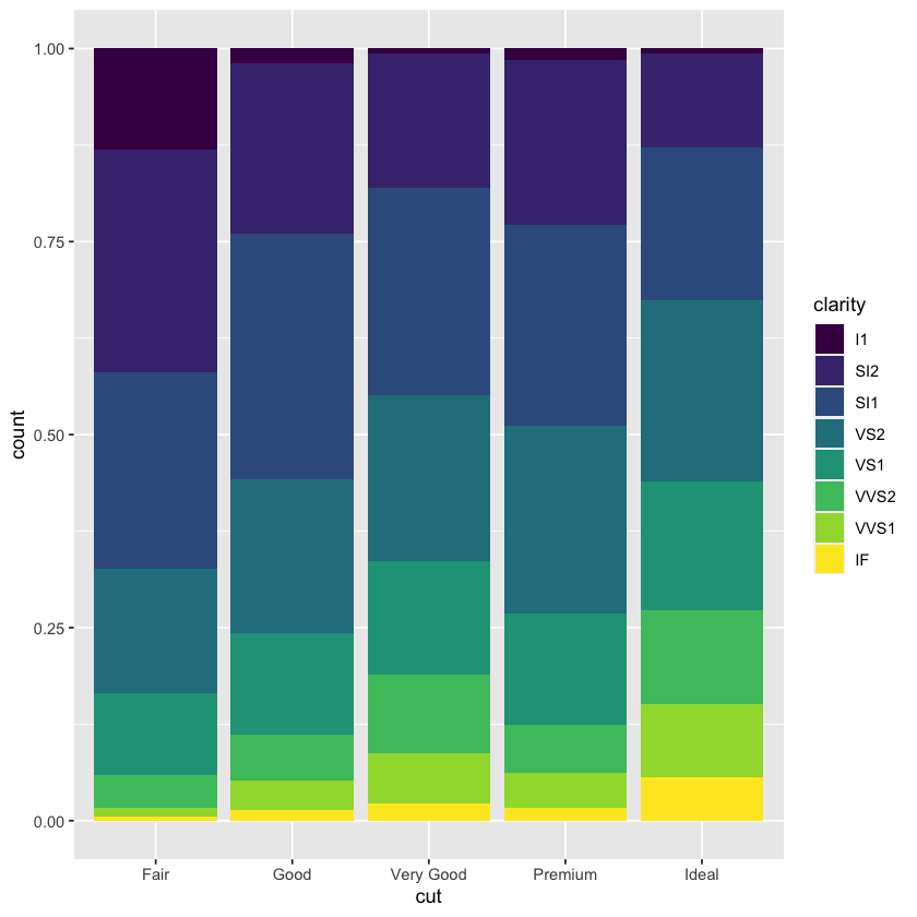
ggplot(data = diamonds) +
  geom_bar(mapping = aes(x = cut, fill = clarity), position = 'fill')
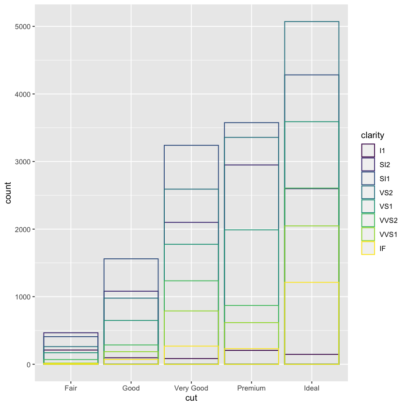
ggplot(data = diamonds, mapping = aes(x = cut, color = clarity)) +
  geom_bar(fill = NA, position = 'identity')
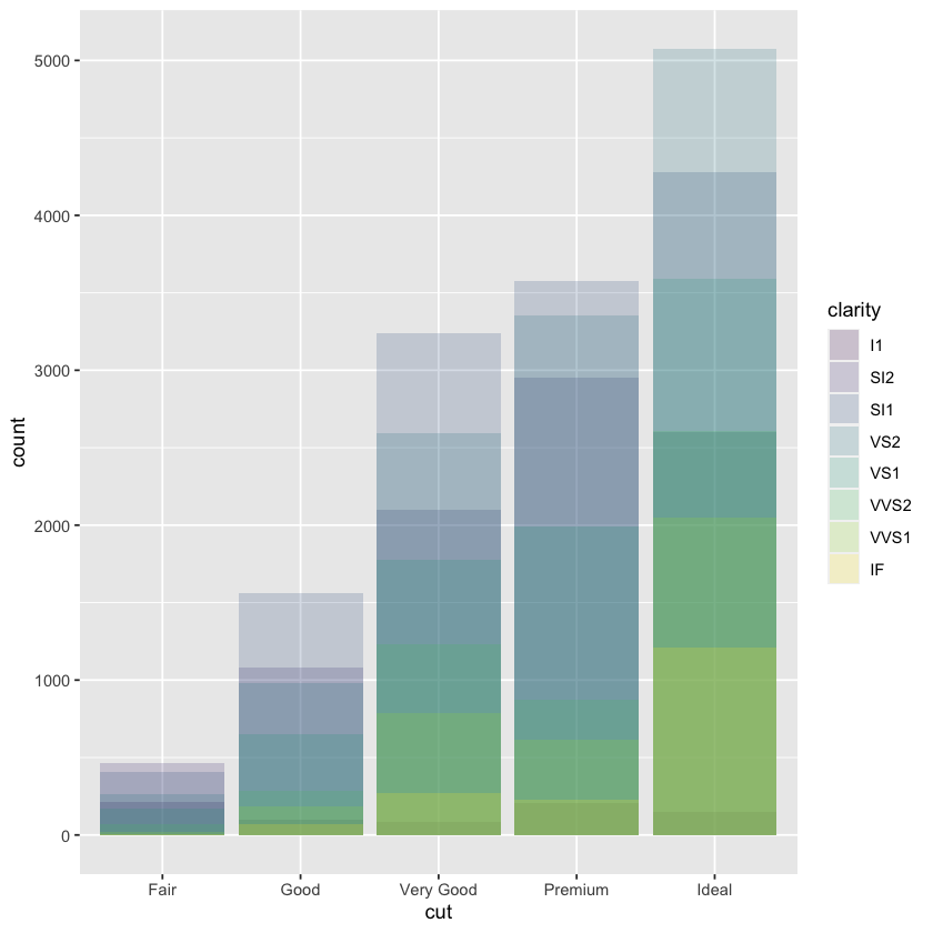
ggplot(data = diamonds, mapping = aes(x = cut, fill = clarity)) +
  geom_bar(alpha = 1/5, position = 'identity')
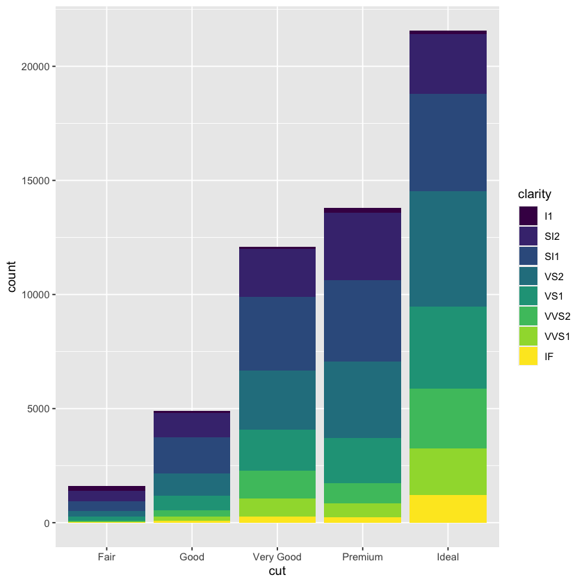
ggplot(data = diamonds) +
  geom_bar(mapping = aes(x = cut, fill = clarity))
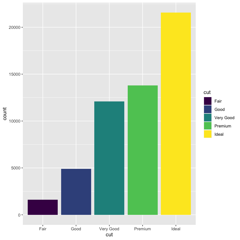
ggplot(data = diamonds) +
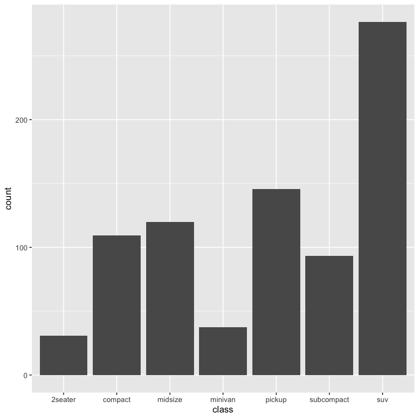
  geom_bar(mapping = aes(x = cut, fill = cut))
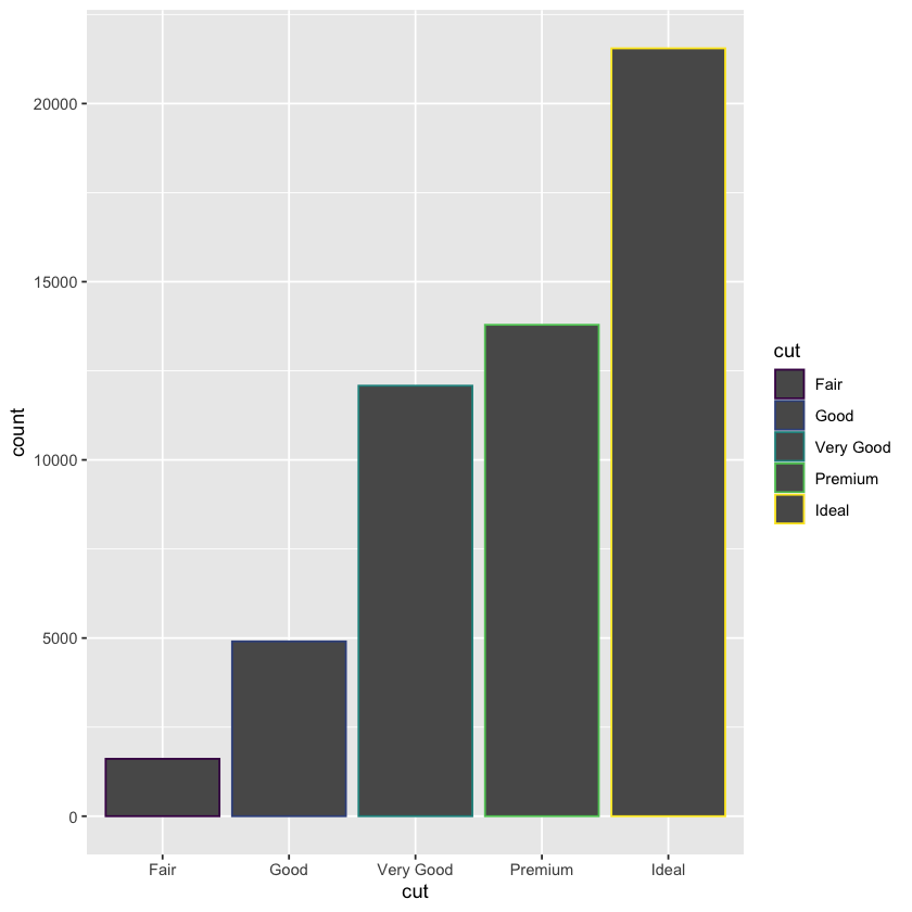
ggplot(data = diamonds) +
  geom_bar(mapping = aes(x = cut, color = cut))

ggplot(data = mpg) +
  geom_point(mapping = aes(x = displ, y = hwy), position = 'jitter')

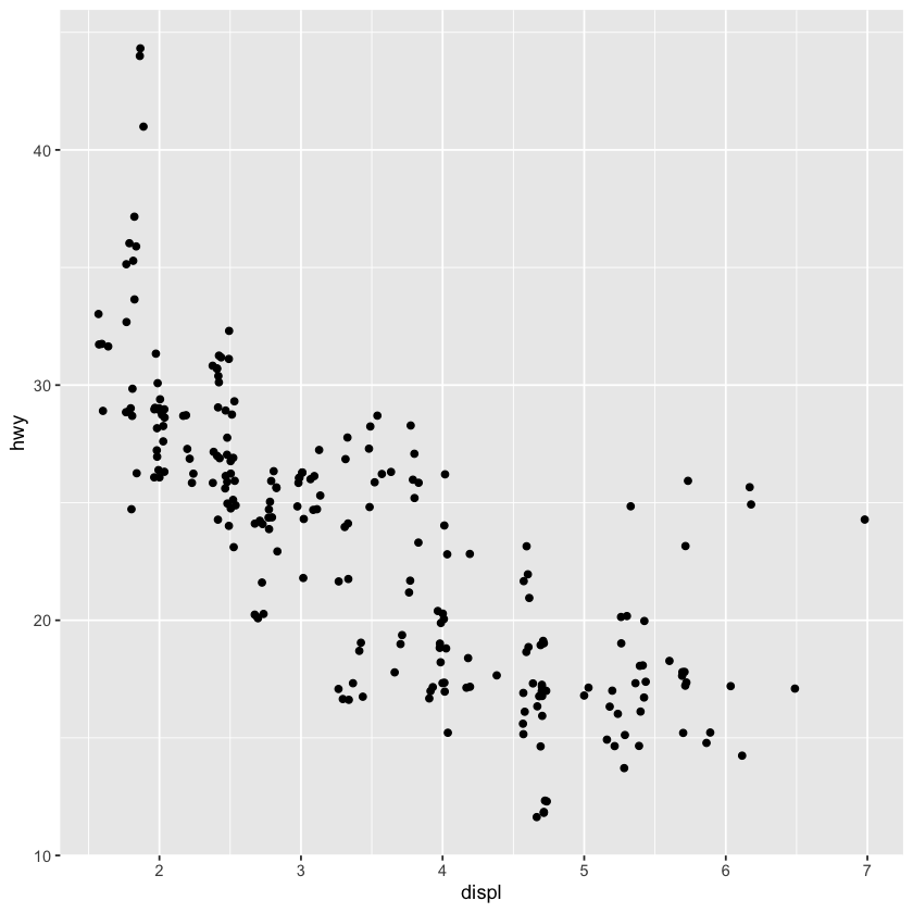
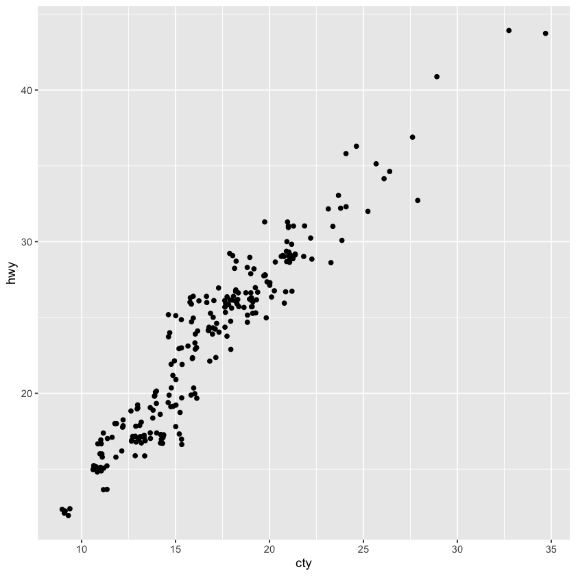
ggplot(data = mpg, mapping = aes(x = cty, y = hwy)) + geom_jitter()
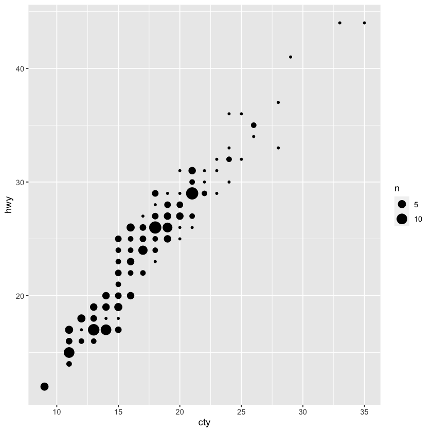
ggplot(data = mpg, mapping = aes(x = cty, y = hwy)) + geom_count()
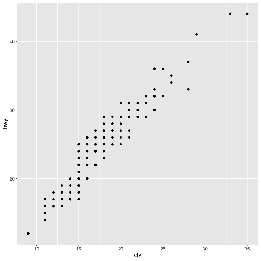
ggplot(data = mpg, mapping = aes(x = cty, y = hwy)) + geom_point()

head(mpg)

A tibble: 6 × 11

manufacturer	model	displ	year	cyl	trans	drv	cty	hwy	fl	class
<chr>	<chr>	<dbl>	<int>	<int>	<chr>	<chr>	<int>	<int>	<chr>	<chr>
audi	a4	1.8	1999	4	auto(l5)	f	18	29	p	compact
audi	a4	1.8	1999	4	manual(m5)	f	21	29	p	compact
audi	a4	2.0	2008	4	manual(m6)	f	20	31	p	compact
audi	a4	2.0	2008	4	auto(av)	f	21	30	p	compact
audi	a4	2.8	1999	6	auto(l5)	f	16	26	p	compact
audi	a4	2.8	1999	6	manual(m5)	f	18	26	p	compact

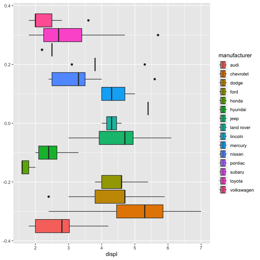
ggplot(data = mpg) +
  geom_boxplot(mapping = aes(x = displ, fill = manufacturer))

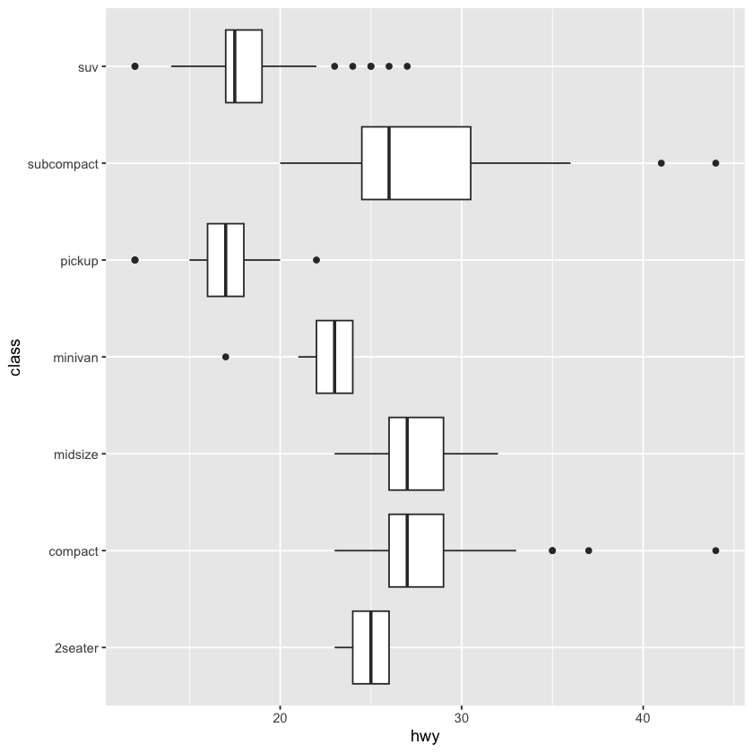
ggplot(data = mpg, mapping = aes(x = class, y = hwy)) + geom_boxplot() + coord_flip()
ggplot(data = mpg, mapping = aes(x = class, y = hwy)) + geom_boxplot()

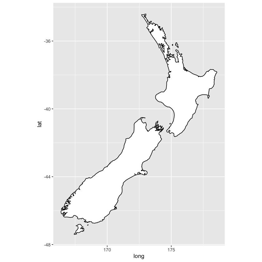
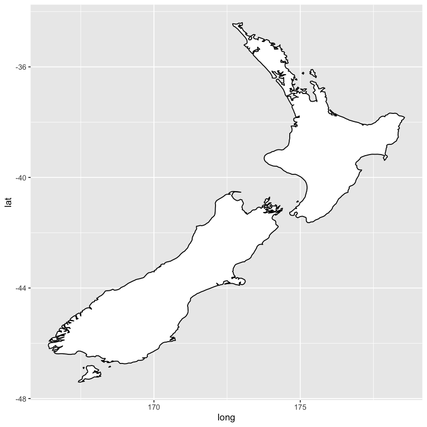
nz <- map_data('nz')
ggplot(data = nz, mapping = aes(x = long, y = lat, group = group)) +
  geom_polygon(fill = 'white', color = 'black') +
  coord_quickmap()
ggplot(data = nz, mapping = aes(x = long, y = lat, group = group)) +
  geom_polygon(fill = 'white', color = 'black')

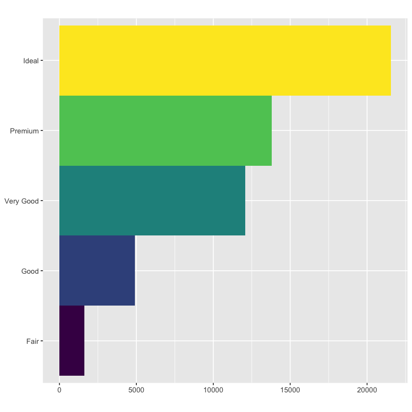
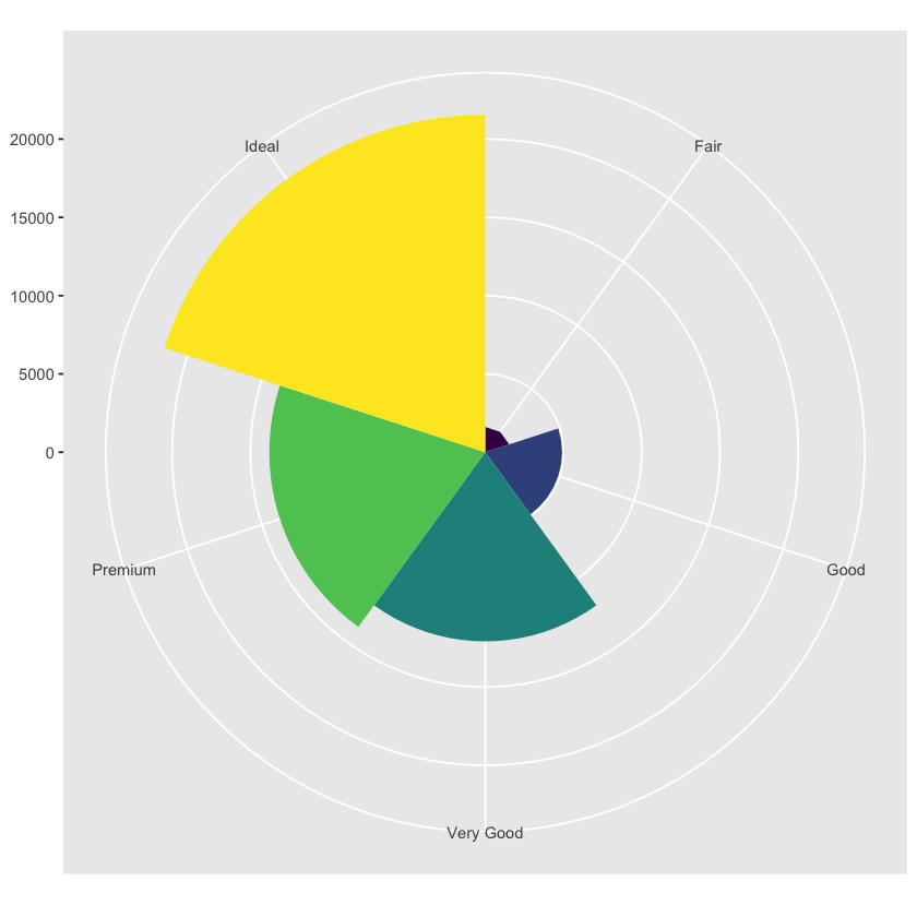
bar <- ggplot(data = diamonds) +
  geom_bar(
    mapping = aes(x = cut, fill = cut),
    show.legend = FALSE,
    width = 1
  ) +
  theme(aspect.ratio = 1) +
  labs(x = NULL, y = NULL)

bar + coord_flip()
bar + coord_polar()

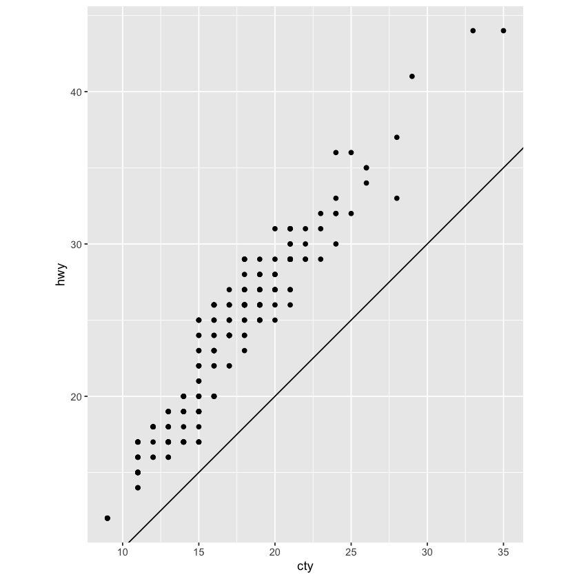
# 3.9.1 [4]

ggplot(data = mpg, mapping = aes(x = cty, y = hwy)) +
  geom_point() +
  geom_abline() +
  coord_fixed()

---

04 - Workflow: basics

sin(pi/2)
seq(1,10)
typeof(seq(1,10))
seq(1,10,length.out=5)
1:10

1

1. 1
2. 2
3. 3
4. 4
5. 5
6. 6
7. 7
8. 8
9. 9
10. 10

'integer'

1. 1
2. 3.25
3. 5.5
4. 7.75
5. 10

1. 1
2. 2
3. 3
4. 4
5. 5
6. 6
7. 7
8. 8
9. 9
10. 10

---

05 - Data Transformation

airlines

A tibble: 16 × 2

carrier	name
<chr>	<chr>
9E	Endeavor Air Inc.
AA	American Airlines Inc.
AS	Alaska Airlines Inc.
B6	JetBlue Airways
DL	Delta Air Lines Inc.
EV	ExpressJet Airlines Inc.
F9	Frontier Airlines Inc.
FL	AirTran Airways Corporation
HA	Hawaiian Airlines Inc.
MQ	Envoy Air
OO	SkyWest Airlines Inc.
UA	United Air Lines Inc.
US	US Airways Inc.
VX	Virgin America
WN	Southwest Airlines Co.
YV	Mesa Airlines Inc.

airports

A tibble: 1458 × 8

faa	name	lat	lon	alt	tz	dst	tzone
<chr>	<chr>	<dbl>	<dbl>	<dbl>	<dbl>	<chr>	<chr>
04G	Lansdowne Airport	41.13047	-80.61958	1044	-5	A	America/New_York
06A	Moton Field Municipal Airport	32.46057	-85.68003	264	-6	A	America/Chicago
06C	Schaumburg Regional	41.98934	-88.10124	801	-6	A	America/Chicago
06N	Randall Airport	41.43191	-74.39156	523	-5	A	America/New_York
09J	Jekyll Island Airport	31.07447	-81.42778	11	-5	A	America/New_York
0A9	Elizabethton Municipal Airport	36.37122	-82.17342	1593	-5	A	America/New_York
0G6	Williams County Airport	41.46731	-84.50678	730	-5	A	America/New_York
0G7	Finger Lakes Regional Airport	42.88356	-76.78123	492	-5	A	America/New_York
0P2	Shoestring Aviation Airfield	39.79482	-76.64719	1000	-5	U	America/New_York
0S9	Jefferson County Intl	48.05381	-122.81064	108	-8	A	America/Los_Angeles
0W3	Harford County Airport	39.56684	-76.20240	409	-5	A	America/New_York
10C	Galt Field Airport	42.40289	-88.37511	875	-6	U	America/Chicago
17G	Port Bucyrus-Crawford County Airport	40.78156	-82.97481	1003	-5	A	America/New_York
19A	Jackson County Airport	34.17586	-83.56160	951	-5	U	America/New_York
1A3	Martin Campbell Field Airport	35.01581	-84.34683	1789	-5	A	America/New_York
1B9	Mansfield Municipal	42.00013	-71.19677	122	-5	A	America/New_York
1C9	Frazier Lake Airpark	54.01333	-124.76833	152	-8	A	America/Vancouver
1CS	Clow International Airport	41.69597	-88.12923	670	-6	U	America/Chicago
1G3	Kent State Airport	41.15139	-81.41511	1134	-5	A	America/New_York
1G4	Grand Canyon West Airport	35.89990	-113.81567	4813	-7	A	America/Phoenix
1H2	Effingham Memorial Airport	39.07000	-88.53400	585	-6	A	America/Chicago
1OH	Fortman Airport	40.55533	-84.38662	885	-5	U	America/New_York
1RL	Point Roberts Airpark	48.97972	-123.07889	10	-8	A	America/Los_Angeles
23M	Clarke CO	32.05170	-88.44340	320	-6	A	America/Chicago
24C	Lowell City Airport	42.95392	-85.34391	681	-5	A	America/New_York
24J	Suwannee County Airport	30.30013	-83.02469	104	-5	A	America/New_York
25D	Forest Lake Airport	45.24775	-92.99439	925	-6	A	America/Chicago
29D	Grove City Airport	41.14603	-80.16775	1371	-5	A	America/New_York
2A0	Mark Anton Airport	35.48625	-84.93108	718	-5	A	America/New_York
2B2	Plum Island Airport	42.79536	-70.83944	11	-5	A	America/New_York
⋮	⋮	⋮	⋮	⋮	⋮	⋮	⋮
X59	Valkaria Municipal	27.96086	-80.55833	26	-5	A	America/New_York
XFL	Flagler County Airport	29.28210	-81.12120	33	-5	A	America/New_York
XNA	NW Arkansas Regional	36.28187	-94.30681	1287	-6	A	America/Chicago
XZK	Amherst Amtrak Station AMM	42.37500	-72.51139	258	-5	A	America/New_York
Y51	Municipal Airport	43.57936	-90.89647	1292	-6	A	America/Chicago
Y72	Bloyer Field	43.97622	-90.48061	966	-6	A	America/Chicago
YAK	Yakutat	59.30120	-139.39370	33	-9	A	NA
YIP	Willow Run	42.23793	-83.53041	716	-5	A	America/New_York
YKM	Yakima Air Terminal McAllister Field	46.56820	-120.54400	1095	-8	A	America/Los_Angeles
YKN	Chan Gurney	42.87110	-97.39690	1200	-6	A	America/Chicago
YNG	Youngstown Warren Rgnl	41.26074	-80.67910	1196	-5	A	America/New_York
YUM	Yuma Mcas Yuma Intl	32.65658	-114.60598	216	-7	N	America/Phoenix
Z84	Clear	64.30120	-149.12014	552	-9	A	America/Anchorage
ZBP	Penn Station	39.30722	-76.61556	66	-5	A	America/New_York
ZFV	Philadelphia 30th St Station	39.95570	-75.18200	0	-5	A	America/New_York
ZPH	Municipal Airport	28.22806	-82.15583	90	-5	A	America/New_York
ZRA	Atlantic City Rail Terminal	39.36650	-74.44200	8	-5	A	America/New_York
ZRD	Train Station	37.53430	-77.42945	26	-5	A	America/New_York
ZRP	Newark Penn Station	40.73472	-74.16417	0	-5	A	America/New_York
ZRT	Hartford Union Station	41.76888	-72.68150	0	-5	A	America/New_York
ZRZ	New Carrollton Rail Station	38.94800	-76.87190	39	-5	A	America/New_York
ZSF	Springfield Amtrak Station	42.10600	-72.59305	65	-5	A	America/New_York
ZSY	Scottsdale Airport	33.62289	-111.91053	1519	-7	A	America/Phoenix
ZTF	Stamford Amtrak Station	41.04694	-73.54149	0	-5	A	America/New_York
ZTY	Boston Back Bay Station	42.34780	-71.07500	20	-5	A	America/New_York
ZUN	Black Rock	35.08323	-108.79178	6454	-7	A	America/Denver
ZVE	New Haven Rail Station	41.29867	-72.92599	7	-5	A	America/New_York
ZWI	Wilmington Amtrak Station	39.73667	-75.55167	0	-5	A	America/New_York
ZWU	Washington Union Station	38.89746	-77.00643	76	-5	A	America/New_York
ZYP	Penn Station	40.75050	-73.99350	35	-5	A	America/New_York

flights

A tibble: 336776 × 19

year	month	day	dep_time	sched_dep_time	dep_delay	arr_time	sched_arr_time	arr_delay	carrier	flight	tailnum	origin	dest	air_time	distance	hour	minute	time_hour
<int>	<int>	<int>	<int>	<int>	<dbl>	<int>	<int>	<dbl>	<chr>	<int>	<chr>	<chr>	<chr>	<dbl>	<dbl>	<dbl>	<dbl>	<dttm>
2013	1	1	517	515	2	830	819	11	UA	1545	N14228	EWR	IAH	227	1400	5	15	2013-01-01 05:00:00
2013	1	1	533	529	4	850	830	20	UA	1714	N24211	LGA	IAH	227	1416	5	29	2013-01-01 05:00:00
2013	1	1	542	540	2	923	850	33	AA	1141	N619AA	JFK	MIA	160	1089	5	40	2013-01-01 05:00:00
2013	1	1	544	545	-1	1004	1022	-18	B6	725	N804JB	JFK	BQN	183	1576	5	45	2013-01-01 05:00:00
2013	1	1	554	600	-6	812	837	-25	DL	461	N668DN	LGA	ATL	116	762	6	0	2013-01-01 06:00:00
2013	1	1	554	558	-4	740	728	12	UA	1696	N39463	EWR	ORD	150	719	5	58	2013-01-01 05:00:00
2013	1	1	555	600	-5	913	854	19	B6	507	N516JB	EWR	FLL	158	1065	6	0	2013-01-01 06:00:00
2013	1	1	557	600	-3	709	723	-14	EV	5708	N829AS	LGA	IAD	53	229	6	0	2013-01-01 06:00:00
2013	1	1	557	600	-3	838	846	-8	B6	79	N593JB	JFK	MCO	140	944	6	0	2013-01-01 06:00:00
2013	1	1	558	600	-2	753	745	8	AA	301	N3ALAA	LGA	ORD	138	733	6	0	2013-01-01 06:00:00
2013	1	1	558	600	-2	849	851	-2	B6	49	N793JB	JFK	PBI	149	1028	6	0	2013-01-01 06:00:00
2013	1	1	558	600	-2	853	856	-3	B6	71	N657JB	JFK	TPA	158	1005	6	0	2013-01-01 06:00:00
2013	1	1	558	600	-2	924	917	7	UA	194	N29129	JFK	LAX	345	2475	6	0	2013-01-01 06:00:00
2013	1	1	558	600	-2	923	937	-14	UA	1124	N53441	EWR	SFO	361	2565	6	0	2013-01-01 06:00:00
2013	1	1	559	600	-1	941	910	31	AA	707	N3DUAA	LGA	DFW	257	1389	6	0	2013-01-01 06:00:00
2013	1	1	559	559	0	702	706	-4	B6	1806	N708JB	JFK	BOS	44	187	5	59	2013-01-01 05:00:00
2013	1	1	559	600	-1	854	902	-8	UA	1187	N76515	EWR	LAS	337	2227	6	0	2013-01-01 06:00:00
2013	1	1	600	600	0	851	858	-7	B6	371	N595JB	LGA	FLL	152	1076	6	0	2013-01-01 06:00:00
2013	1	1	600	600	0	837	825	12	MQ	4650	N542MQ	LGA	ATL	134	762	6	0	2013-01-01 06:00:00
2013	1	1	601	600	1	844	850	-6	B6	343	N644JB	EWR	PBI	147	1023	6	0	2013-01-01 06:00:00
2013	1	1	602	610	-8	812	820	-8	DL	1919	N971DL	LGA	MSP	170	1020	6	10	2013-01-01 06:00:00
2013	1	1	602	605	-3	821	805	16	MQ	4401	N730MQ	LGA	DTW	105	502	6	5	2013-01-01 06:00:00
2013	1	1	606	610	-4	858	910	-12	AA	1895	N633AA	EWR	MIA	152	1085	6	10	2013-01-01 06:00:00
2013	1	1	606	610	-4	837	845	-8	DL	1743	N3739P	JFK	ATL	128	760	6	10	2013-01-01 06:00:00
2013	1	1	607	607	0	858	915	-17	UA	1077	N53442	EWR	MIA	157	1085	6	7	2013-01-01 06:00:00
2013	1	1	608	600	8	807	735	32	MQ	3768	N9EAMQ	EWR	ORD	139	719	6	0	2013-01-01 06:00:00
2013	1	1	611	600	11	945	931	14	UA	303	N532UA	JFK	SFO	366	2586	6	0	2013-01-01 06:00:00
2013	1	1	613	610	3	925	921	4	B6	135	N635JB	JFK	RSW	175	1074	6	10	2013-01-01 06:00:00
2013	1	1	615	615	0	1039	1100	-21	B6	709	N794JB	JFK	SJU	182	1598	6	15	2013-01-01 06:00:00
2013	1	1	615	615	0	833	842	-9	DL	575	N326NB	EWR	ATL	120	746	6	15	2013-01-01 06:00:00
⋮	⋮	⋮	⋮	⋮	⋮	⋮	⋮	⋮	⋮	⋮	⋮	⋮	⋮	⋮	⋮	⋮	⋮	⋮
2013	9	30	2123	2125	-2	2223	2247	-24	EV	5489	N712EV	LGA	CHO	45	305	21	25	2013-09-30 21:00:00
2013	9	30	2127	2129	-2	2314	2323	-9	EV	3833	N16546	EWR	CLT	72	529	21	29	2013-09-30 21:00:00
2013	9	30	2128	2130	-2	2328	2359	-31	B6	97	N807JB	JFK	DEN	213	1626	21	30	2013-09-30 21:00:00
2013	9	30	2129	2059	30	2230	2232	-2	EV	5048	N751EV	LGA	RIC	45	292	20	59	2013-09-30 20:00:00
2013	9	30	2131	2140	-9	2225	2255	-30	MQ	3621	N807MQ	JFK	DCA	36	213	21	40	2013-09-30 21:00:00
2013	9	30	2140	2140	0	10	40	-30	AA	185	N335AA	JFK	LAX	298	2475	21	40	2013-09-30 21:00:00
2013	9	30	2142	2129	13	2250	2239	11	EV	4509	N12957	EWR	PWM	47	284	21	29	2013-09-30 21:00:00
2013	9	30	2145	2145	0	115	140	-25	B6	1103	N633JB	JFK	SJU	192	1598	21	45	2013-09-30 21:00:00
2013	9	30	2147	2137	10	30	27	3	B6	1371	N627JB	LGA	FLL	139	1076	21	37	2013-09-30 21:00:00
2013	9	30	2149	2156	-7	2245	2308	-23	UA	523	N813UA	EWR	BOS	37	200	21	56	2013-09-30 21:00:00
2013	9	30	2150	2159	-9	2250	2306	-16	EV	3842	N10575	EWR	MHT	39	209	21	59	2013-09-30 21:00:00
2013	9	30	2159	1845	194	2344	2030	194	9E	3320	N906XJ	JFK	BUF	50	301	18	45	2013-09-30 18:00:00
2013	9	30	2203	2205	-2	2339	2331	8	EV	5311	N722EV	LGA	BGR	61	378	22	5	2013-09-30 22:00:00
2013	9	30	2207	2140	27	2257	2250	7	MQ	3660	N532MQ	LGA	BNA	97	764	21	40	2013-09-30 21:00:00
2013	9	30	2211	2059	72	2339	2242	57	EV	4672	N12145	EWR	STL	120	872	20	59	2013-09-30 20:00:00
2013	9	30	2231	2245	-14	2335	2356	-21	B6	108	N193JB	JFK	PWM	48	273	22	45	2013-09-30 22:00:00
2013	9	30	2233	2113	80	112	30	42	UA	471	N578UA	EWR	SFO	318	2565	21	13	2013-09-30 21:00:00
2013	9	30	2235	2001	154	59	2249	130	B6	1083	N804JB	JFK	MCO	123	944	20	1	2013-09-30 20:00:00
2013	9	30	2237	2245	-8	2345	2353	-8	B6	234	N318JB	JFK	BTV	43	266	22	45	2013-09-30 22:00:00
2013	9	30	2240	2245	-5	2334	2351	-17	B6	1816	N354JB	JFK	SYR	41	209	22	45	2013-09-30 22:00:00
2013	9	30	2240	2250	-10	2347	7	-20	B6	2002	N281JB	JFK	BUF	52	301	22	50	2013-09-30 22:00:00
2013	9	30	2241	2246	-5	2345	1	-16	B6	486	N346JB	JFK	ROC	47	264	22	46	2013-09-30 22:00:00
2013	9	30	2307	2255	12	2359	2358	1	B6	718	N565JB	JFK	BOS	33	187	22	55	2013-09-30 22:00:00
2013	9	30	2349	2359	-10	325	350	-25	B6	745	N516JB	JFK	PSE	196	1617	23	59	2013-09-30 23:00:00
2013	9	30	NA	1842	NA	NA	2019	NA	EV	5274	N740EV	LGA	BNA	NA	764	18	42	2013-09-30 18:00:00
2013	9	30	NA	1455	NA	NA	1634	NA	9E	3393	NA	JFK	DCA	NA	213	14	55	2013-09-30 14:00:00
2013	9	30	NA	2200	NA	NA	2312	NA	9E	3525	NA	LGA	SYR	NA	198	22	0	2013-09-30 22:00:00
2013	9	30	NA	1210	NA	NA	1330	NA	MQ	3461	N535MQ	LGA	BNA	NA	764	12	10	2013-09-30 12:00:00
2013	9	30	NA	1159	NA	NA	1344	NA	MQ	3572	N511MQ	LGA	CLE	NA	419	11	59	2013-09-30 11:00:00
2013	9	30	NA	840	NA	NA	1020	NA	MQ	3531	N839MQ	LGA	RDU	NA	431	8	40	2013-09-30 08:00:00

weather

A tibble: 26115 × 15

origin	year	month	day	hour	temp	dewp	humid	wind_dir	wind_speed	wind_gust	precip	pressure	visib	time_hour
<chr>	<int>	<int>	<int>	<int>	<dbl>	<dbl>	<dbl>	<dbl>	<dbl>	<dbl>	<dbl>	<dbl>	<dbl>	<dttm>
EWR	2013	1	1	1	39.02	26.06	59.37	270	10.35702	NA	0	1012.0	10	2013-01-01 01:00:00
EWR	2013	1	1	2	39.02	26.96	61.63	250	8.05546	NA	0	1012.3	10	2013-01-01 02:00:00
EWR	2013	1	1	3	39.02	28.04	64.43	240	11.50780	NA	0	1012.5	10	2013-01-01 03:00:00
EWR	2013	1	1	4	39.92	28.04	62.21	250	12.65858	NA	0	1012.2	10	2013-01-01 04:00:00
EWR	2013	1	1	5	39.02	28.04	64.43	260	12.65858	NA	0	1011.9	10	2013-01-01 05:00:00
EWR	2013	1	1	6	37.94	28.04	67.21	240	11.50780	NA	0	1012.4	10	2013-01-01 06:00:00
EWR	2013	1	1	7	39.02	28.04	64.43	240	14.96014	NA	0	1012.2	10	2013-01-01 07:00:00
EWR	2013	1	1	8	39.92	28.04	62.21	250	10.35702	NA	0	1012.2	10	2013-01-01 08:00:00
EWR	2013	1	1	9	39.92	28.04	62.21	260	14.96014	NA	0	1012.7	10	2013-01-01 09:00:00
EWR	2013	1	1	10	41.00	28.04	59.65	260	13.80936	NA	0	1012.4	10	2013-01-01 10:00:00
EWR	2013	1	1	11	41.00	26.96	57.06	260	14.96014	NA	0	1011.4	10	2013-01-01 11:00:00
EWR	2013	1	1	13	39.20	28.40	69.67	330	16.11092	NA	0	NA	10	2013-01-01 13:00:00
EWR	2013	1	1	14	39.02	24.08	54.68	280	13.80936	NA	0	1010.8	10	2013-01-01 14:00:00
EWR	2013	1	1	15	37.94	24.08	57.04	290	9.20624	NA	0	1011.9	10	2013-01-01 15:00:00
EWR	2013	1	1	16	37.04	19.94	49.62	300	13.80936	20.71404	0	1012.1	10	2013-01-01 16:00:00
EWR	2013	1	1	17	35.96	19.04	49.83	330	11.50780	NA	0	1013.2	10	2013-01-01 17:00:00
EWR	2013	1	1	18	33.98	15.08	45.43	310	12.65858	25.31716	0	1014.1	10	2013-01-01 18:00:00
EWR	2013	1	1	19	33.08	12.92	42.84	320	10.35702	NA	0	1014.4	10	2013-01-01 19:00:00
EWR	2013	1	1	20	32.00	15.08	49.19	310	14.96014	NA	0	1015.2	10	2013-01-01 20:00:00
EWR	2013	1	1	21	30.02	12.92	48.48	320	18.41248	26.46794	0	1016.0	10	2013-01-01 21:00:00
EWR	2013	1	1	22	28.94	12.02	48.69	320	18.41248	25.31716	0	1016.5	10	2013-01-01 22:00:00
EWR	2013	1	1	23	28.04	10.94	48.15	310	16.11092	NA	0	1016.4	10	2013-01-01 23:00:00
EWR	2013	1	2	0	26.96	10.94	50.34	310	14.96014	25.31716	0	1016.3	10	2013-01-02 00:00:00
EWR	2013	1	2	1	26.06	10.94	52.25	330	12.65858	24.16638	0	1016.3	10	2013-01-02 01:00:00
EWR	2013	1	2	2	24.98	10.94	54.65	330	13.80936	NA	0	1017.0	10	2013-01-02 02:00:00
EWR	2013	1	2	3	24.08	8.96	51.93	320	14.96014	NA	0	1016.6	10	2013-01-02 03:00:00
EWR	2013	1	2	4	24.08	8.96	51.93	330	12.65858	NA	0	1016.9	10	2013-01-02 04:00:00
EWR	2013	1	2	5	24.08	8.96	51.93	330	6.90468	NA	0	1016.9	10	2013-01-02 05:00:00
EWR	2013	1	2	6	24.08	8.96	51.93	310	3.45234	NA	0	1017.2	10	2013-01-02 06:00:00
EWR	2013	1	2	7	24.98	10.04	52.50	300	6.90468	NA	0	1017.6	10	2013-01-02 07:00:00
⋮	⋮	⋮	⋮	⋮	⋮	⋮	⋮	⋮	⋮	⋮	⋮	⋮	⋮	⋮
LGA	2013	12	29	13	42.80	37.94	88.76	70	12.65858	NA	0.19	NA	2.50	2013-12-29 13:00:00
LGA	2013	12	29	14	41.00	37.94	93.19	60	18.41248	NA	0.21	NA	1.75	2013-12-29 14:00:00
LGA	2013	12	29	15	41.00	39.02	92.59	40	13.80936	NA	0.37	999.9	1.50	2013-12-29 15:00:00
LGA	2013	12	29	16	41.00	37.94	88.76	350	8.05546	23.01560	0.28	998.7	1.50	2013-12-29 16:00:00
LGA	2013	12	29	17	44.06	41.00	93.24	350	20.71404	NA	0.04	NA	5.00	2013-12-29 17:00:00
LGA	2013	12	29	18	42.08	39.02	88.81	330	14.96014	NA	0.00	997.2	3.00	2013-12-29 18:00:00
LGA	2013	12	29	19	42.80	37.94	85.13	320	17.26170	NA	0.00	NA	8.00	2013-12-29 19:00:00
LGA	2013	12	29	20	42.08	37.94	86.89	320	19.56326	NA	0.00	NA	10.00	2013-12-29 20:00:00
LGA	2013	12	29	21	42.80	37.40	82.17	320	16.11092	NA	0.00	NA	10.00	2013-12-29 21:00:00
LGA	2013	12	29	22	42.98	37.04	79.38	300	9.20624	NA	0.00	1003.8	10.00	2013-12-29 22:00:00
LGA	2013	12	29	23	42.98	35.06	73.39	310	17.26170	24.16638	0.00	1005.1	10.00	2013-12-29 23:00:00
LGA	2013	12	30	0	42.08	33.98	72.78	320	11.50780	NA	0.00	1005.9	10.00	2013-12-30 00:00:00
LGA	2013	12	30	1	42.08	33.98	72.78	250	9.20624	NA	0.00	1007.6	10.00	2013-12-30 01:00:00
LGA	2013	12	30	2	41.00	33.98	75.88	240	8.05546	NA	0.00	1008.3	10.00	2013-12-30 02:00:00
LGA	2013	12	30	3	42.98	33.98	70.30	270	9.20624	NA	0.00	1008.2	10.00	2013-12-30 03:00:00
LGA	2013	12	30	4	41.00	33.08	73.19	0	0.00000	NA	0.00	1008.9	10.00	2013-12-30 04:00:00
LGA	2013	12	30	5	42.98	33.08	67.81	250	10.35702	NA	0.00	1009.2	10.00	2013-12-30 05:00:00
LGA	2013	12	30	6	42.98	33.98	70.30	230	6.90468	NA	0.00	1010.8	10.00	2013-12-30 06:00:00
LGA	2013	12	30	7	44.06	35.06	70.42	240	11.50780	NA	0.00	1011.9	10.00	2013-12-30 07:00:00
LGA	2013	12	30	8	44.06	33.98	67.45	260	11.50780	NA	0.00	1012.9	10.00	2013-12-30 08:00:00
LGA	2013	12	30	9	44.06	33.08	65.07	260	13.80936	NA	0.00	1013.7	10.00	2013-12-30 09:00:00
LGA	2013	12	30	10	42.98	33.80	70.28	330	16.11092	NA	0.00	NA	10.00	2013-12-30 10:00:00
LGA	2013	12	30	11	41.00	28.40	62.21	340	13.80936	23.01560	0.00	NA	10.00	2013-12-30 11:00:00
LGA	2013	12	30	12	37.94	23.00	54.51	330	21.86482	27.61872	0.00	1015.7	10.00	2013-12-30 12:00:00
LGA	2013	12	30	13	37.04	21.92	53.97	340	17.26170	20.71404	0.00	1016.5	10.00	2013-12-30 13:00:00
LGA	2013	12	30	14	35.96	19.94	51.78	340	13.80936	21.86482	0.00	1017.1	10.00	2013-12-30 14:00:00
LGA	2013	12	30	15	33.98	17.06	49.51	330	17.26170	21.86482	0.00	1018.8	10.00	2013-12-30 15:00:00
LGA	2013	12	30	16	32.00	15.08	49.19	340	14.96014	23.01560	0.00	1019.5	10.00	2013-12-30 16:00:00
LGA	2013	12	30	17	30.92	12.92	46.74	320	17.26170	NA	0.00	1019.9	10.00	2013-12-30 17:00:00
LGA	2013	12	30	18	28.94	10.94	46.41	330	18.41248	NA	0.00	1020.9	10.00	2013-12-30 18:00:00

flights %>%
  count(month)

A tibble: 12 × 2

month	n
<int>	<int>
1	27004
2	24951
3	28834
4	28330
5	28796
6	28243
7	29425
8	29327
9	27574
10	28889
11	27268
12	28135

vars <- c('year','month','day','dep_delay','arr_delay')
flights %>%
  #filter(arr_delay >= 2)                             # 1.1. Find all flights that had an arrival delay of two or more hours
  #filter(dest %in% c('IAH','HOU'))                   # 1.2. Find all flights that flew to Houston (IAH or HOU)
  #filter(carrier %in% c('AA','DL','UA'))             # 1.3. Find all flights that were operated by United, American, or Delta
  #filter(month %in% c(7,8,9))                        # 1.4. Find all flights that departed in summer (July, August, and September)
  #filter(arr_delay > 120 & dep_delay <= 0)           # 1.5. Find all flights that arrived more than two hours late, but didn't leave late.
  #filter(dep_delay >= 60 & arr_delay < dep_delay-30) # 1.6. Find all flights that were delayed by at least an hour, but made up over 30 minutes in flight.
  #filter(dep_time >= 1 & dep_time <= 600)            # 1.7. Find all flights that departed between midnight and 6am (inclusive).
  #filter(between(dep_time, 1, 600))                  # 2.
  #filter(is.na(dep_time))                            # 3.
  #arrange(desc(is.na(dep_delay)))                    # 5.3.1 [1] How could you use arrange() to sort all missing values to the start? (Hint: use is.na())
  #arrange(desc(dep_delay))                           # 5.3.1 [2] Sort flights to find the most delayed flights. Find the flights that left earliest.
  #arrange(desc(distance/air_time))                   # 5.3.1 [3] Sort flights to find the fastest (highest speed) flights.
  #arrange(desc(distance))                            # 5.3.1 [4] Which flights travelled the farthest? Which travelled the shortest?
  #select(year,month,day)                             # Select columns by name
  #select(year:day)                                   # Select all columns between year and day (inclusive)
  #select(-(year:day))                                # Select all columns except those from year to day (inclusive)
  #rename(tail_num = tailnum)
  #select(time_hour, air_time, everything())          # Move a handful of variables to the start of the data frame.
  #select(dep_delay,dep_delay,dep_delay,arr_delay)    # 5.4.1 [2] What happens if you include the name of a variable multiple times in a select() call?
  #select(any_of(vars))                               # 5.4.1 [3] What does the any_of() function do? Why might it be helpful in conjunction with vector `vars`?
  select(contains('TIME'))                           # 5.4.1 [4] Does the result of running this code surprise you? How do the select helpers deal with case by default? How can you change that default?

A tibble: 336776 × 6

dep_time	sched_dep_time	arr_time	sched_arr_time	air_time	time_hour
<int>	<int>	<int>	<int>	<dbl>	<dttm>
517	515	830	819	227	2013-01-01 05:00:00
533	529	850	830	227	2013-01-01 05:00:00
542	540	923	850	160	2013-01-01 05:00:00
544	545	1004	1022	183	2013-01-01 05:00:00
554	600	812	837	116	2013-01-01 06:00:00
554	558	740	728	150	2013-01-01 05:00:00
555	600	913	854	158	2013-01-01 06:00:00
557	600	709	723	53	2013-01-01 06:00:00
557	600	838	846	140	2013-01-01 06:00:00
558	600	753	745	138	2013-01-01 06:00:00
558	600	849	851	149	2013-01-01 06:00:00
558	600	853	856	158	2013-01-01 06:00:00
558	600	924	917	345	2013-01-01 06:00:00
558	600	923	937	361	2013-01-01 06:00:00
559	600	941	910	257	2013-01-01 06:00:00
559	559	702	706	44	2013-01-01 05:00:00
559	600	854	902	337	2013-01-01 06:00:00
600	600	851	858	152	2013-01-01 06:00:00
600	600	837	825	134	2013-01-01 06:00:00
601	600	844	850	147	2013-01-01 06:00:00
602	610	812	820	170	2013-01-01 06:00:00
602	605	821	805	105	2013-01-01 06:00:00
606	610	858	910	152	2013-01-01 06:00:00
606	610	837	845	128	2013-01-01 06:00:00
607	607	858	915	157	2013-01-01 06:00:00
608	600	807	735	139	2013-01-01 06:00:00
611	600	945	931	366	2013-01-01 06:00:00
613	610	925	921	175	2013-01-01 06:00:00
615	615	1039	1100	182	2013-01-01 06:00:00
615	615	833	842	120	2013-01-01 06:00:00
⋮	⋮	⋮	⋮	⋮	⋮
2123	2125	2223	2247	45	2013-09-30 21:00:00
2127	2129	2314	2323	72	2013-09-30 21:00:00
2128	2130	2328	2359	213	2013-09-30 21:00:00
2129	2059	2230	2232	45	2013-09-30 20:00:00
2131	2140	2225	2255	36	2013-09-30 21:00:00
2140	2140	10	40	298	2013-09-30 21:00:00
2142	2129	2250	2239	47	2013-09-30 21:00:00
2145	2145	115	140	192	2013-09-30 21:00:00
2147	2137	30	27	139	2013-09-30 21:00:00
2149	2156	2245	2308	37	2013-09-30 21:00:00
2150	2159	2250	2306	39	2013-09-30 21:00:00
2159	1845	2344	2030	50	2013-09-30 18:00:00
2203	2205	2339	2331	61	2013-09-30 22:00:00
2207	2140	2257	2250	97	2013-09-30 21:00:00
2211	2059	2339	2242	120	2013-09-30 20:00:00
2231	2245	2335	2356	48	2013-09-30 22:00:00
2233	2113	112	30	318	2013-09-30 21:00:00
2235	2001	59	2249	123	2013-09-30 20:00:00
2237	2245	2345	2353	43	2013-09-30 22:00:00
2240	2245	2334	2351	41	2013-09-30 22:00:00
2240	2250	2347	7	52	2013-09-30 22:00:00
2241	2246	2345	1	47	2013-09-30 22:00:00
2307	2255	2359	2358	33	2013-09-30 22:00:00
2349	2359	325	350	196	2013-09-30 23:00:00
NA	1842	NA	2019	NA	2013-09-30 18:00:00
NA	1455	NA	1634	NA	2013-09-30 14:00:00
NA	2200	NA	2312	NA	2013-09-30 22:00:00
NA	1210	NA	1330	NA	2013-09-30 12:00:00
NA	1159	NA	1344	NA	2013-09-30 11:00:00
NA	840	NA	1020	NA	2013-09-30 08:00:00

flights_sml <- flights %>%
  select(
    year:day,
    ends_with('delay'),
    distance,
    air_time
  )
flights_sml %>%
  mutate(
    gain          = dep_delay - arr_delay,
    hours         = air_time / 60,
    gain_per_hour = gain / hours,
    speed         = distance / air_time * 60
  )
flights %>%
  transmute(
    gain          = dep_delay - arr_delay,
    hours         = air_time / 60,
    gain_per_hour = gain / hours
  )

A tibble: 336776 × 11

year	month	day	dep_delay	arr_delay	distance	air_time	gain	hours	gain_per_hour	speed
<int>	<int>	<int>	<dbl>	<dbl>	<dbl>	<dbl>	<dbl>	<dbl>	<dbl>	<dbl>
2013	1	1	2	11	1400	227	-9	3.7833333	-2.3788546	370.0441
2013	1	1	4	20	1416	227	-16	3.7833333	-4.2290749	374.2731
2013	1	1	2	33	1089	160	-31	2.6666667	-11.6250000	408.3750
2013	1	1	-1	-18	1576	183	17	3.0500000	5.5737705	516.7213
2013	1	1	-6	-25	762	116	19	1.9333333	9.8275862	394.1379
2013	1	1	-4	12	719	150	-16	2.5000000	-6.4000000	287.6000
2013	1	1	-5	19	1065	158	-24	2.6333333	-9.1139241	404.4304
2013	1	1	-3	-14	229	53	11	0.8833333	12.4528302	259.2453
2013	1	1	-3	-8	944	140	5	2.3333333	2.1428571	404.5714
2013	1	1	-2	8	733	138	-10	2.3000000	-4.3478261	318.6957
2013	1	1	-2	-2	1028	149	0	2.4833333	0.0000000	413.9597
2013	1	1	-2	-3	1005	158	1	2.6333333	0.3797468	381.6456
2013	1	1	-2	7	2475	345	-9	5.7500000	-1.5652174	430.4348
2013	1	1	-2	-14	2565	361	12	6.0166667	1.9944598	426.3158
2013	1	1	-1	31	1389	257	-32	4.2833333	-7.4708171	324.2802
2013	1	1	0	-4	187	44	4	0.7333333	5.4545455	255.0000
2013	1	1	-1	-8	2227	337	7	5.6166667	1.2462908	396.4985
2013	1	1	0	-7	1076	152	7	2.5333333	2.7631579	424.7368
2013	1	1	0	12	762	134	-12	2.2333333	-5.3731343	341.1940
2013	1	1	1	-6	1023	147	7	2.4500000	2.8571429	417.5510
2013	1	1	-8	-8	1020	170	0	2.8333333	0.0000000	360.0000
2013	1	1	-3	16	502	105	-19	1.7500000	-10.8571429	286.8571
2013	1	1	-4	-12	1085	152	8	2.5333333	3.1578947	428.2895
2013	1	1	-4	-8	760	128	4	2.1333333	1.8750000	356.2500
2013	1	1	0	-17	1085	157	17	2.6166667	6.4968153	414.6497
2013	1	1	8	32	719	139	-24	2.3166667	-10.3597122	310.3597
2013	1	1	11	14	2586	366	-3	6.1000000	-0.4918033	423.9344
2013	1	1	3	4	1074	175	-1	2.9166667	-0.3428571	368.2286
2013	1	1	0	-21	1598	182	21	3.0333333	6.9230769	526.8132
2013	1	1	0	-9	746	120	9	2.0000000	4.5000000	373.0000
⋮	⋮	⋮	⋮	⋮	⋮	⋮	⋮	⋮	⋮	⋮
2013	9	30	-2	-24	305	45	22	0.7500000	29.333333	406.6667
2013	9	30	-2	-9	529	72	7	1.2000000	5.833333	440.8333
2013	9	30	-2	-31	1626	213	29	3.5500000	8.169014	458.0282
2013	9	30	30	-2	292	45	32	0.7500000	42.666667	389.3333
2013	9	30	-9	-30	213	36	21	0.6000000	35.000000	355.0000
2013	9	30	0	-30	2475	298	30	4.9666667	6.040268	498.3221
2013	9	30	13	11	284	47	2	0.7833333	2.553191	362.5532
2013	9	30	0	-25	1598	192	25	3.2000000	7.812500	499.3750
2013	9	30	10	3	1076	139	7	2.3166667	3.021583	464.4604
2013	9	30	-7	-23	200	37	16	0.6166667	25.945946	324.3243
2013	9	30	-9	-16	209	39	7	0.6500000	10.769231	321.5385
2013	9	30	194	194	301	50	0	0.8333333	0.000000	361.2000
2013	9	30	-2	8	378	61	-10	1.0166667	-9.836066	371.8033
2013	9	30	27	7	764	97	20	1.6166667	12.371134	472.5773
2013	9	30	72	57	872	120	15	2.0000000	7.500000	436.0000
2013	9	30	-14	-21	273	48	7	0.8000000	8.750000	341.2500
2013	9	30	80	42	2565	318	38	5.3000000	7.169811	483.9623
2013	9	30	154	130	944	123	24	2.0500000	11.707317	460.4878
2013	9	30	-8	-8	266	43	0	0.7166667	0.000000	371.1628
2013	9	30	-5	-17	209	41	12	0.6833333	17.560976	305.8537
2013	9	30	-10	-20	301	52	10	0.8666667	11.538462	347.3077
2013	9	30	-5	-16	264	47	11	0.7833333	14.042553	337.0213
2013	9	30	12	1	187	33	11	0.5500000	20.000000	340.0000
2013	9	30	-10	-25	1617	196	15	3.2666667	4.591837	495.0000
2013	9	30	NA	NA	764	NA	NA	NA	NA	NA
2013	9	30	NA	NA	213	NA	NA	NA	NA	NA
2013	9	30	NA	NA	198	NA	NA	NA	NA	NA
2013	9	30	NA	NA	764	NA	NA	NA	NA	NA
2013	9	30	NA	NA	419	NA	NA	NA	NA	NA
2013	9	30	NA	NA	431	NA	NA	NA	NA	NA

A tibble: 336776 × 3

gain	hours	gain_per_hour
<dbl>	<dbl>	<dbl>
-9	3.7833333	-2.3788546
-16	3.7833333	-4.2290749
-31	2.6666667	-11.6250000
17	3.0500000	5.5737705
19	1.9333333	9.8275862
-16	2.5000000	-6.4000000
-24	2.6333333	-9.1139241
11	0.8833333	12.4528302
5	2.3333333	2.1428571
-10	2.3000000	-4.3478261
0	2.4833333	0.0000000
1	2.6333333	0.3797468
-9	5.7500000	-1.5652174
12	6.0166667	1.9944598
-32	4.2833333	-7.4708171
4	0.7333333	5.4545455
7	5.6166667	1.2462908
7	2.5333333	2.7631579
-12	2.2333333	-5.3731343
7	2.4500000	2.8571429
0	2.8333333	0.0000000
-19	1.7500000	-10.8571429
8	2.5333333	3.1578947
4	2.1333333	1.8750000
17	2.6166667	6.4968153
-24	2.3166667	-10.3597122
-3	6.1000000	-0.4918033
-1	2.9166667	-0.3428571
21	3.0333333	6.9230769
9	2.0000000	4.5000000
⋮	⋮	⋮
22	0.7500000	29.333333
7	1.2000000	5.833333
29	3.5500000	8.169014
32	0.7500000	42.666667
21	0.6000000	35.000000
30	4.9666667	6.040268
2	0.7833333	2.553191
25	3.2000000	7.812500
7	2.3166667	3.021583
16	0.6166667	25.945946
7	0.6500000	10.769231
0	0.8333333	0.000000
-10	1.0166667	-9.836066
20	1.6166667	12.371134
15	2.0000000	7.500000
7	0.8000000	8.750000
38	5.3000000	7.169811
24	2.0500000	11.707317
0	0.7166667	0.000000
12	0.6833333	17.560976
10	0.8666667	11.538462
11	0.7833333	14.042553
11	0.5500000	20.000000
15	3.2666667	4.591837
NA	NA	NA
NA	NA	NA
NA	NA	NA
NA	NA	NA
NA	NA	NA
NA	NA	NA

flights %>% head(2)

A tibble: 2 × 19

year	month	day	dep_time	sched_dep_time	dep_delay	arr_time	sched_arr_time	arr_delay	carrier	flight	tailnum	origin	dest	air_time	distance	hour	minute	time_hour
<int>	<int>	<int>	<int>	<int>	<dbl>	<int>	<int>	<dbl>	<chr>	<int>	<chr>	<chr>	<chr>	<dbl>	<dbl>	<dbl>	<dbl>	<dttm>
2013	1	1	517	515	2	830	819	11	UA	1545	N14228	EWR	IAH	227	1400	5	15	2013-01-01 05:00:00
2013	1	1	533	529	4	850	830	20	UA	1714	N24211	LGA	IAH	227	1416	5	29	2013-01-01 05:00:00

flights %>%
  transmute(
             dep_time,
    hour   = dep_time %/% 100,
    minute = dep_time %% 100
  )

A tibble: 336776 × 3

dep_time	hour	minute
<int>	<dbl>	<dbl>
517	5	17
533	5	33
542	5	42
544	5	44
554	5	54
554	5	54
555	5	55
557	5	57
557	5	57
558	5	58
558	5	58
558	5	58
558	5	58
558	5	58
559	5	59
559	5	59
559	5	59
600	6	0
600	6	0
601	6	1
602	6	2
602	6	2
606	6	6
606	6	6
607	6	7
608	6	8
611	6	11
613	6	13
615	6	15
615	6	15
⋮	⋮	⋮
2123	21	23
2127	21	27
2128	21	28
2129	21	29
2131	21	31
2140	21	40
2142	21	42
2145	21	45
2147	21	47
2149	21	49
2150	21	50
2159	21	59
2203	22	3
2207	22	7
2211	22	11
2231	22	31
2233	22	33
2235	22	35
2237	22	37
2240	22	40
2240	22	40
2241	22	41
2307	23	7
2349	23	49
NA	NA	NA
NA	NA	NA
NA	NA	NA
NA	NA	NA
NA	NA	NA
NA	NA	NA

(x <- 1:10)
lag(x)
lead(x)
cumsum(x)
cumprod(x)
cummin(x)
cummax(x)
cummean(x)

1. 1
2. 2
3. 3
4. 4
5. 5
6. 6
7. 7
8. 8
9. 9
10. 10

1. <NA>
2. 1
3. 2
4. 3
5. 4
6. 5
7. 6
8. 7
9. 8
10. 9

1. 2
2. 3
3. 4
4. 5
5. 6
6. 7
7. 8
8. 9
9. 10
10. <NA>

1. 1
2. 3
3. 6
4. 10
5. 15
6. 21
7. 28
8. 36
9. 45
10. 55

1. 1
2. 2
3. 6
4. 24
5. 120
6. 720
7. 5040
8. 40320
9. 362880
10. 3628800

1. 1
2. 1
3. 1
4. 1
5. 1
6. 1
7. 1
8. 1
9. 1
10. 1

1. 1
2. 2
3. 3
4. 4
5. 5
6. 6
7. 7
8. 8
9. 9
10. 10

1. 1
2. 1.5
3. 2
4. 2.5
5. 3
6. 3.5
7. 4
8. 4.5
9. 5
10. 5.5

y <- c(1,2,2,NA,3,4)
min_rank(y)
min_rank(desc(y))
row_number(y)
dense_rank(y)
percent_rank(y)
cume_dist(y)

1. 1
2. 2
3. 2
4. <NA>
5. 4
6. 5

1. 5
2. 3
3. 3
4. <NA>
5. 2
6. 1

1. 1
2. 2
3. 3
4. <NA>
5. 4
6. 5

1. 1
2. 2
3. 2
4. <NA>
5. 3
6. 4

1. 0
2. 0.25
3. 0.25
4. <NA>
5. 0.75
6. 1

1. 0.2
2. 0.6
3. 0.6
4. <NA>
5. 0.8
6. 1

# 5.5.2 [1] Currently `dep_time` and `sched_dep_time` are convenient to look at, but hard to compute with because they're not really continuous numbers. Convert them to a more convenient representation of number of minutes since midnight.

flights %>%
  transmute(
                         sched_dep_time,
    sched_dep_time_min = sched_dep_time %/% 100 * 60 + sched_dep_time %% 100,
                               dep_time,
          dep_time_min =       dep_time %/% 100 * 60 +       dep_time %% 100
  )

A tibble: 336776 × 4

sched_dep_time	sched_dep_time_min	dep_time	dep_time_min
<int>	<dbl>	<int>	<dbl>
515	315	517	317
529	329	533	333
540	340	542	342
545	345	544	344
600	360	554	354
558	358	554	354
600	360	555	355
600	360	557	357
600	360	557	357
600	360	558	358
600	360	558	358
600	360	558	358
600	360	558	358
600	360	558	358
600	360	559	359
559	359	559	359
600	360	559	359
600	360	600	360
600	360	600	360
600	360	601	361
610	370	602	362
605	365	602	362
610	370	606	366
610	370	606	366
607	367	607	367
600	360	608	368
600	360	611	371
610	370	613	373
615	375	615	375
615	375	615	375
⋮	⋮	⋮	⋮
2125	1285	2123	1283
2129	1289	2127	1287
2130	1290	2128	1288
2059	1259	2129	1289
2140	1300	2131	1291
2140	1300	2140	1300
2129	1289	2142	1302
2145	1305	2145	1305
2137	1297	2147	1307
2156	1316	2149	1309
2159	1319	2150	1310
1845	1125	2159	1319
2205	1325	2203	1323
2140	1300	2207	1327
2059	1259	2211	1331
2245	1365	2231	1351
2113	1273	2233	1353
2001	1201	2235	1355
2245	1365	2237	1357
2245	1365	2240	1360
2250	1370	2240	1360
2246	1366	2241	1361
2255	1375	2307	1387
2359	1439	2349	1429
1842	1122	NA	NA
1455	895	NA	NA
2200	1320	NA	NA
1210	730	NA	NA
1159	719	NA	NA
840	520	NA	NA

# 5.5.2 [2] Compare `air_time` with `arr_time - dep_time`. What do you expect to see? What do you see? What do you need to do to fix it?

flights %>%
  transmute(
    air_time,
    dep_time_min = dep_time %/% 100 * 60 + dep_time %% 100,
    arr_time_min = arr_time %/% 100 * 60 + arr_time %% 100,
    air_time_min = arr_time_min - dep_time_min,
    TZdelta      = air_time_min - air_time
  )

A tibble: 336776 × 5

air_time	dep_time_min	arr_time_min	air_time_min	TZdelta
<dbl>	<dbl>	<dbl>	<dbl>	<dbl>
227	317	510	193	-34
227	333	530	197	-30
160	342	563	221	61
183	344	604	260	77
116	354	492	138	22
150	354	460	106	-44
158	355	553	198	40
53	357	429	72	19
140	357	518	161	21
138	358	473	115	-23
149	358	529	171	22
158	358	533	175	17
345	358	564	206	-139
361	358	563	205	-156
257	359	581	222	-35
44	359	422	63	19
337	359	534	175	-162
152	360	531	171	19
134	360	517	157	23
147	361	524	163	16
170	362	492	130	-40
105	362	501	139	34
152	366	538	172	20
128	366	517	151	23
157	367	538	171	14
139	368	487	119	-20
366	371	585	214	-152
175	373	565	192	17
182	375	639	264	82
120	375	513	138	18
⋮	⋮	⋮	⋮	⋮
45	1283	1343	60	15
72	1287	1394	107	35
213	1288	1408	120	-93
45	1289	1350	61	16
36	1291	1345	54	18
298	1300	10	-1290	-1588
47	1302	1370	68	21
192	1305	75	-1230	-1422
139	1307	30	-1277	-1416
37	1309	1365	56	19
39	1310	1370	60	21
50	1319	1424	105	55
61	1323	1419	96	35
97	1327	1377	50	-47
120	1331	1419	88	-32
48	1351	1415	64	16
318	1353	72	-1281	-1599
123	1355	59	-1296	-1419
43	1357	1425	68	25
41	1360	1414	54	13
52	1360	1427	67	15
47	1361	1425	64	17
33	1387	1439	52	19
196	1429	205	-1224	-1420
NA	NA	NA	NA	NA
NA	NA	NA	NA	NA
NA	NA	NA	NA	NA
NA	NA	NA	NA	NA
NA	NA	NA	NA	NA
NA	NA	NA	NA	NA

# 5.5.2 [3] Compare `dep_time`, `sched_dep_time`, and `dep_delay`. How would you expect those three numbers to be related?

flights %>%
  transmute(
          dep_time_min =       dep_time %/% 100 * 60 +       dep_time %% 100,
    sched_dep_time_min = sched_dep_time %/% 100 * 60 + sched_dep_time %% 100,
    dep_time_min - sched_dep_time_min,
    dep_delay
  )

A tibble: 336776 × 4

dep_time_min	sched_dep_time_min	dep_time_min - sched_dep_time_min	dep_delay
<dbl>	<dbl>	<dbl>	<dbl>
317	315	2	2
333	329	4	4
342	340	2	2
344	345	-1	-1
354	360	-6	-6
354	358	-4	-4
355	360	-5	-5
357	360	-3	-3
357	360	-3	-3
358	360	-2	-2
358	360	-2	-2
358	360	-2	-2
358	360	-2	-2
358	360	-2	-2
359	360	-1	-1
359	359	0	0
359	360	-1	-1
360	360	0	0
360	360	0	0
361	360	1	1
362	370	-8	-8
362	365	-3	-3
366	370	-4	-4
366	370	-4	-4
367	367	0	0
368	360	8	8
371	360	11	11
373	370	3	3
375	375	0	0
375	375	0	0
⋮	⋮	⋮	⋮
1283	1285	-2	-2
1287	1289	-2	-2
1288	1290	-2	-2
1289	1259	30	30
1291	1300	-9	-9
1300	1300	0	0
1302	1289	13	13
1305	1305	0	0
1307	1297	10	10
1309	1316	-7	-7
1310	1319	-9	-9
1319	1125	194	194
1323	1325	-2	-2
1327	1300	27	27
1331	1259	72	72
1351	1365	-14	-14
1353	1273	80	80
1355	1201	154	154
1357	1365	-8	-8
1360	1365	-5	-5
1360	1370	-10	-10
1361	1366	-5	-5
1387	1375	12	12
1429	1439	-10	-10
NA	1122	NA	NA
NA	895	NA	NA
NA	1320	NA	NA
NA	730	NA	NA
NA	719	NA	NA
NA	520	NA	NA

# 5.5.2 [4] Find the 10 most delayed flights using a ranking function. How do you want to handle ties? Carefully read the documentation for min_rank().

flights %>%
  mutate(
    dep_delay_rank = min_rank(desc(dep_delay))
  ) %>%
    arrange(desc(dep_delay)) %>%
      select(dep_delay, dep_delay_rank, everything()) %>%
        head(10)

A tibble: 10 × 20

dep_delay	dep_delay_rank	year	month	day	dep_time	sched_dep_time	arr_time	sched_arr_time	arr_delay	carrier	flight	tailnum	origin	dest	air_time	distance	hour	minute	time_hour
<dbl>	<int>	<int>	<int>	<int>	<int>	<int>	<int>	<int>	<dbl>	<chr>	<int>	<chr>	<chr>	<chr>	<dbl>	<dbl>	<dbl>	<dbl>	<dttm>
1301	1	2013	1	9	641	900	1242	1530	1272	HA	51	N384HA	JFK	HNL	640	4983	9	0	2013-01-09 09:00:00
1137	2	2013	6	15	1432	1935	1607	2120	1127	MQ	3535	N504MQ	JFK	CMH	74	483	19	35	2013-06-15 19:00:00
1126	3	2013	1	10	1121	1635	1239	1810	1109	MQ	3695	N517MQ	EWR	ORD	111	719	16	35	2013-01-10 16:00:00
1014	4	2013	9	20	1139	1845	1457	2210	1007	AA	177	N338AA	JFK	SFO	354	2586	18	45	2013-09-20 18:00:00
1005	5	2013	7	22	845	1600	1044	1815	989	MQ	3075	N665MQ	JFK	CVG	96	589	16	0	2013-07-22 16:00:00
960	6	2013	4	10	1100	1900	1342	2211	931	DL	2391	N959DL	JFK	TPA	139	1005	19	0	2013-04-10 19:00:00
911	7	2013	3	17	2321	810	135	1020	915	DL	2119	N927DA	LGA	MSP	167	1020	8	10	2013-03-17 08:00:00
899	8	2013	6	27	959	1900	1236	2226	850	DL	2007	N3762Y	JFK	PDX	313	2454	19	0	2013-06-27 19:00:00
898	9	2013	7	22	2257	759	121	1026	895	DL	2047	N6716C	LGA	ATL	109	762	7	59	2013-07-22 07:00:00
896	10	2013	12	5	756	1700	1058	2020	878	AA	172	N5DMAA	EWR	MIA	149	1085	17	0	2013-12-05 17:00:00

# 5.5.2 [5] What does `1:3 + 1:10` return? Why?

1:3 + 1:10

Warning message in 1:3 + 1:10:
“longer object length is not a multiple of shorter object length”

1. 2
2. 4
3. 6
4. 5
5. 7
6. 9
7. 8
8. 10
9. 12
10. 11

---

07 - Exploratory Data Analysis

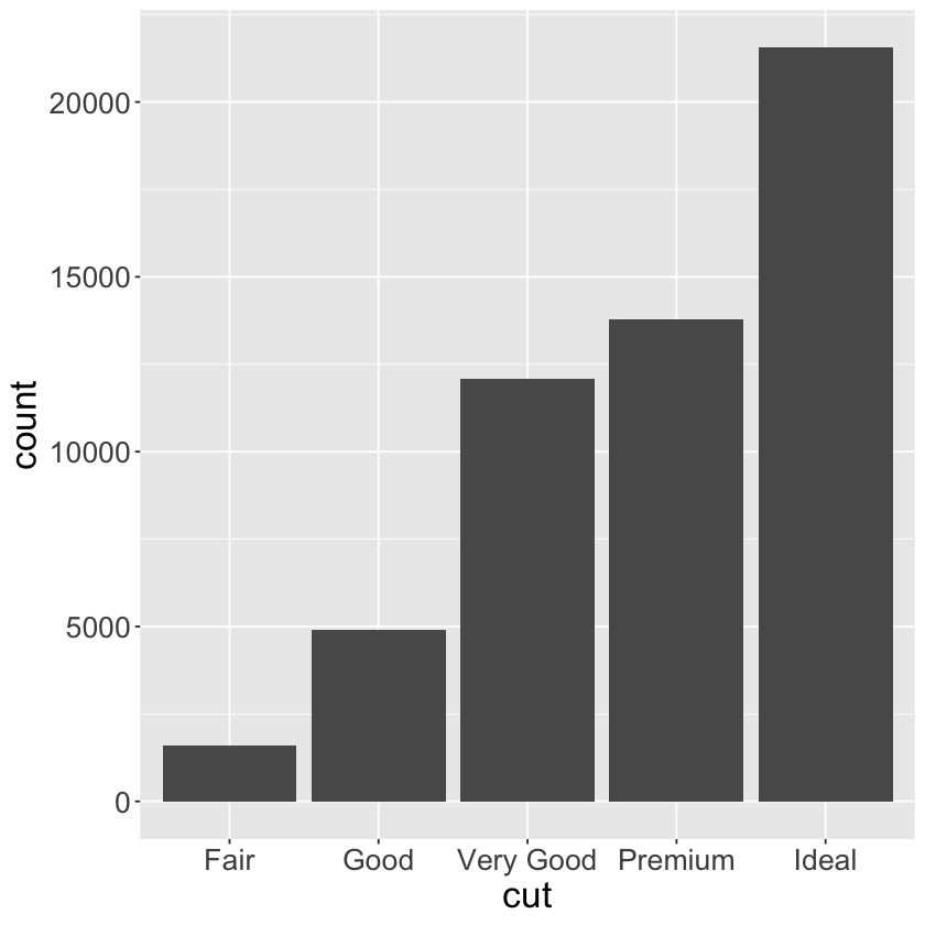
diamonds %>%
  count(cut)

ggplot(data = diamonds) +
  geom_bar(mapping = aes(x = cut)) +
  theme(text = element_text(size = 20))

A tibble: 5 × 2

cut	n
<ord>	<int>
Fair	1610
Good	4906
Very Good	12082
Premium	13791
Ideal	21551

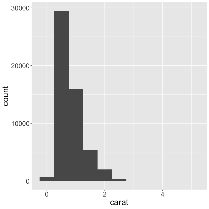
diamonds %>%
  count(cut_width(x = carat, width = 0.5))

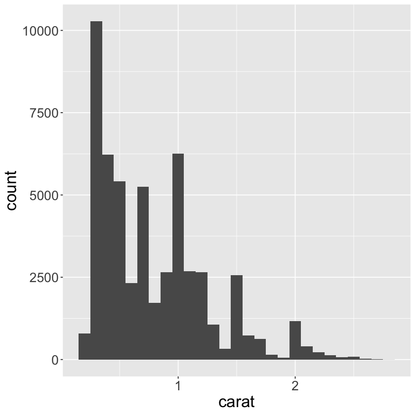
ggplot(data = diamonds) +
  geom_histogram(mapping = aes(x = carat), binwidth = 0.5) +
  theme(text = element_text(size = 20))

A tibble: 11 × 2

cut_width(x = carat, width = 0.5)	n
<fct>	<int>
[-0.25,0.25]	785
(0.25,0.75]	29498
(0.75,1.25]	15977
(1.25,1.75]	5313
(1.75,2.25]	2002
(2.25,2.75]	322
(2.75,3.25]	32
(3.25,3.75]	5
(3.75,4.25]	4
(4.25,4.75]	1
(4.75,5.25]	1

smaller <-
  diamonds %>%
    filter(carat < 3)

smaller %>%
  count(cut_width(x = carat, width = 0.1))

ggplot(data = smaller) +
  geom_histogram(mapping = aes(x = carat), binwidth = 0.1) +
  theme(text = element_text(size = 20))

A tibble: 27 × 2

cut_width(x = carat, width = 0.1)	n
<fct>	<int>
[0.15,0.25]	785
(0.25,0.35]	10273
(0.35,0.45]	6231
(0.45,0.55]	5417
(0.55,0.65]	2328
(0.65,0.75]	5249
(0.75,0.85]	1725
(0.85,0.95]	2656
(0.95,1.05]	6258
(1.05,1.15]	2687
(1.15,1.25]	2651
(1.25,1.35]	1063
(1.35,1.45]	325
(1.45,1.55]	2556
(1.55,1.65]	738
(1.65,1.75]	631
(1.75,1.85]	140
(1.85,1.95]	57
(1.95,2.05]	1173
(2.05,2.15]	407
(2.15,2.25]	225
(2.25,2.35]	135
(2.35,2.45]	69
(2.45,2.55]	81
(2.55,2.65]	21
(2.65,2.75]	16
(2.75,2.85]	3

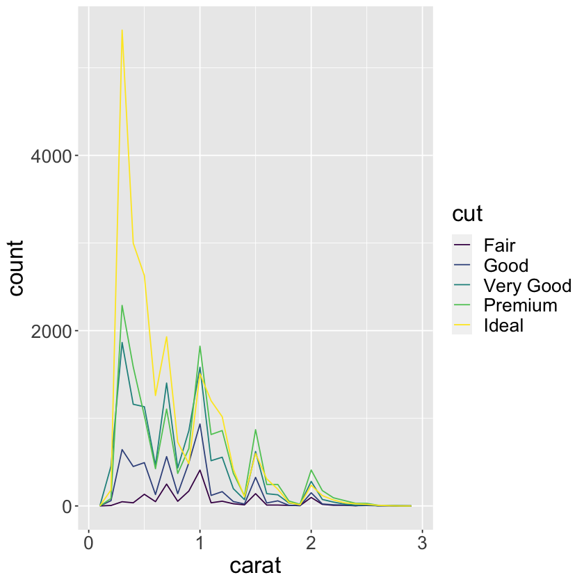
ggplot(data = smaller, mapping = aes(x = carat, color = cut)) +
  geom_freqpoly(binwidth = 0.1) +
  theme(text = element_text(size = 20))

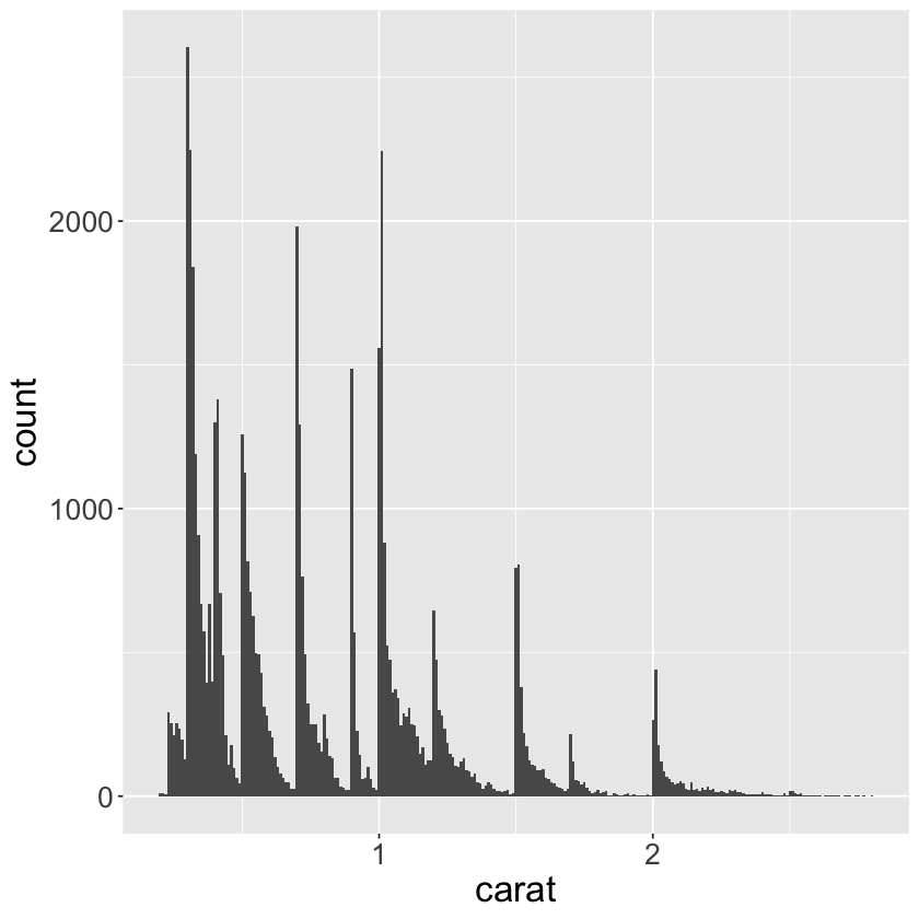
ggplot(data = smaller, mapping = aes(x = carat)) +
  geom_histogram(binwidth = 0.01) +
  theme(text = element_text(size = 20))

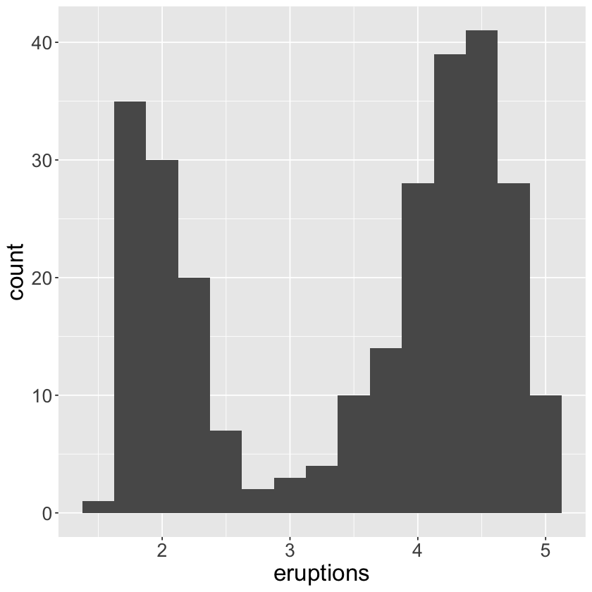
ggplot(data = faithful, mapping = aes(x = eruptions)) +
  geom_histogram(binwidth = 0.25) +
  theme(text = element_text(size = 20))

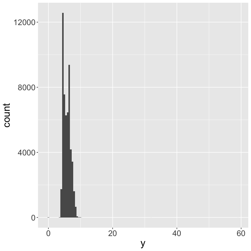
ggplot(data = diamonds) +
  geom_histogram(mapping = aes(x = y), binwidth = 0.5) +
  theme(text = element_text(size = 20))

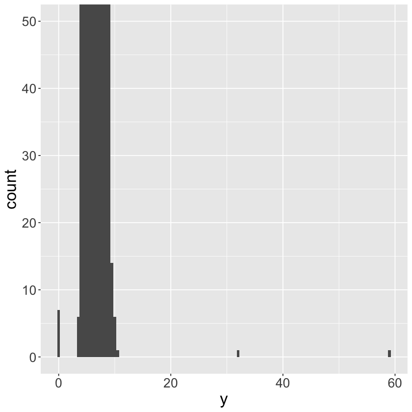
ggplot(data = diamonds) +
  geom_histogram(mapping = aes(x = y), binwidth = 0.5) +
  coord_cartesian(ylim = c(0, 50)) +
  theme(text = element_text(size = 20))

unusual <-
  diamonds %>%
    filter(y < 3 | y > 20) %>%
    select(price, x, y, z) %>%
    arrange(y)
unusual

A tibble: 9 × 4

price	x	y	z
<int>	<dbl>	<dbl>	<dbl>
5139	0.00	0.0	0.00
6381	0.00	0.0	0.00
12800	0.00	0.0	0.00
15686	0.00	0.0	0.00
18034	0.00	0.0	0.00
2130	0.00	0.0	0.00
2130	0.00	0.0	0.00
2075	5.15	31.8	5.12
12210	8.09	58.9	8.06

7.4 - Missing values

Drop the unusual values

diamonds2 <-
  diamonds %>%
    filter(between(x = y, left = 3, right = 20))
head(x = diamonds2)

A tibble: 6 × 10

carat	cut	color	clarity	depth	table	price	x	y	z
<dbl>	<ord>	<ord>	<ord>	<dbl>	<dbl>	<int>	<dbl>	<dbl>	<dbl>
0.23	Ideal	E	SI2	61.5	55	326	3.95	3.98	2.43
0.21	Premium	E	SI1	59.8	61	326	3.89	3.84	2.31
0.23	Good	E	VS1	56.9	65	327	4.05	4.07	2.31
0.29	Premium	I	VS2	62.4	58	334	4.20	4.23	2.63
0.31	Good	J	SI2	63.3	58	335	4.34	4.35	2.75
0.24	Very Good	J	VVS2	62.8	57	336	3.94	3.96	2.48

Replace the unusual values with missing values

diamonds2 <-
  diamonds %>%
    mutate(y = ifelse(test = y < 3 | y > 20, yes = NA, no = y))
head(x = diamonds2)

A tibble: 6 × 10

carat	cut	color	clarity	depth	table	price	x	y	z
<dbl>	<ord>	<ord>	<ord>	<dbl>	<dbl>	<int>	<dbl>	<dbl>	<dbl>
0.23	Ideal	E	SI2	61.5	55	326	3.95	3.98	2.43
0.21	Premium	E	SI1	59.8	61	326	3.89	3.84	2.31
0.23	Good	E	VS1	56.9	65	327	4.05	4.07	2.31
0.29	Premium	I	VS2	62.4	58	334	4.20	4.23	2.63
0.31	Good	J	SI2	63.3	58	335	4.34	4.35	2.75
0.24	Very Good	J	VVS2	62.8	57	336	3.94	3.96	2.48

diamonds2 <-
  diamonds %>%
    mutate(y = case_when(y >= 3 & y <= 20 ~ y, .default = NA))
head(x = diamonds2)

A tibble: 6 × 10

carat	cut	color	clarity	depth	table	price	x	y	z
<dbl>	<ord>	<ord>	<ord>	<dbl>	<dbl>	<int>	<dbl>	<dbl>	<dbl>
0.23	Ideal	E	SI2	61.5	55	326	3.95	3.98	2.43
0.21	Premium	E	SI1	59.8	61	326	3.89	3.84	2.31
0.23	Good	E	VS1	56.9	65	327	4.05	4.07	2.31
0.29	Premium	I	VS2	62.4	58	334	4.20	4.23	2.63
0.31	Good	J	SI2	63.3	58	335	4.34	4.35	2.75
0.24	Very Good	J	VVS2	62.8	57	336	3.94	3.96	2.48

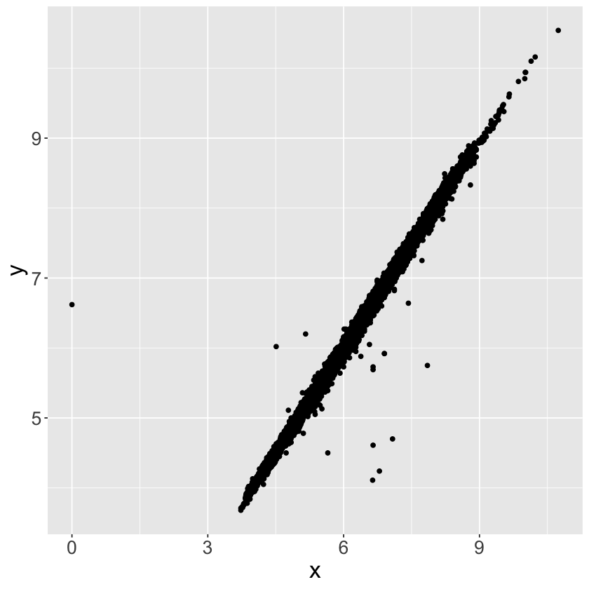
ggplot(data = diamonds2, mapping = aes(x = x, y = y)) +
  geom_point(na.rm = TRUE) +
  theme(text = element_text(size = 20))

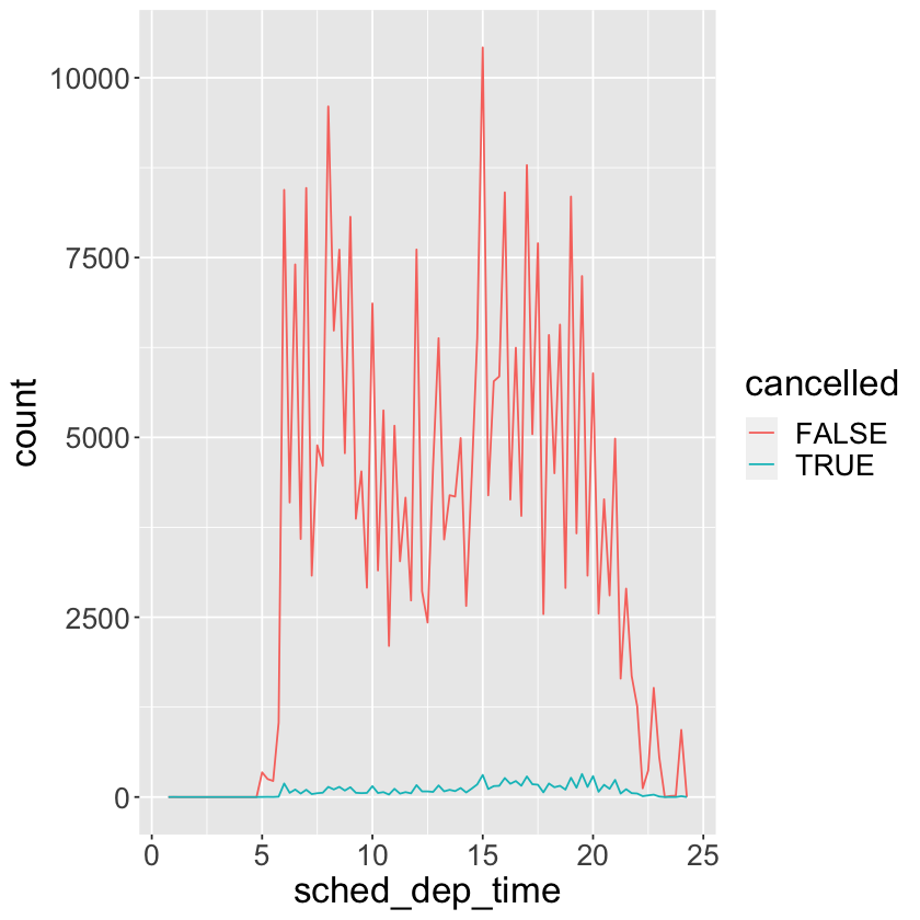
nycflights13::flights %>%
  mutate(
    cancelled      = is.na(dep_time),
    sched_hour     = sched_dep_time %/% 100,
    sched_min      = sched_dep_time %%  100,
    sched_dep_time = sched_hour + sched_min / 60
  ) %>%
    ggplot(mapping = aes(sched_dep_time)) +
      geom_freqpoly(mapping = aes(color = cancelled), binwidth = 1/4) +
      theme(text = element_text(size = 20))

7.5 - Covariation

7.5.1 - One categorical variable and one continuous variable

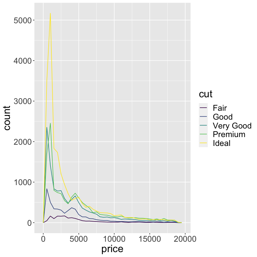
ggplot(data = diamonds, mapping = aes(x = price)) +
  geom_freqpoly(mapping = aes(color = cut), binwidth = 500) +
  theme(text = element_text(size = 20))

ggplot(data = diamonds) +
  geom_bar(mapping = aes(x = cut)) +
  theme(text = element_text(size = 20))

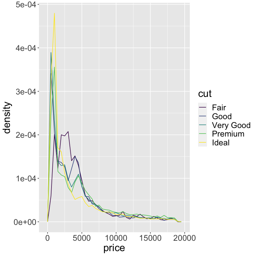
ggplot(data = diamonds, mapping = aes(x = price, y = ..density..)) +
  geom_freqpoly(mapping = aes(color = cut), binwidth = 500) +
  theme(text = element_text(size = 20))

Warning message:
“The dot-dot notation (`..density..`) was deprecated in ggplot2 3.4.0.
ℹ Please use `after_stat(density)` instead.”

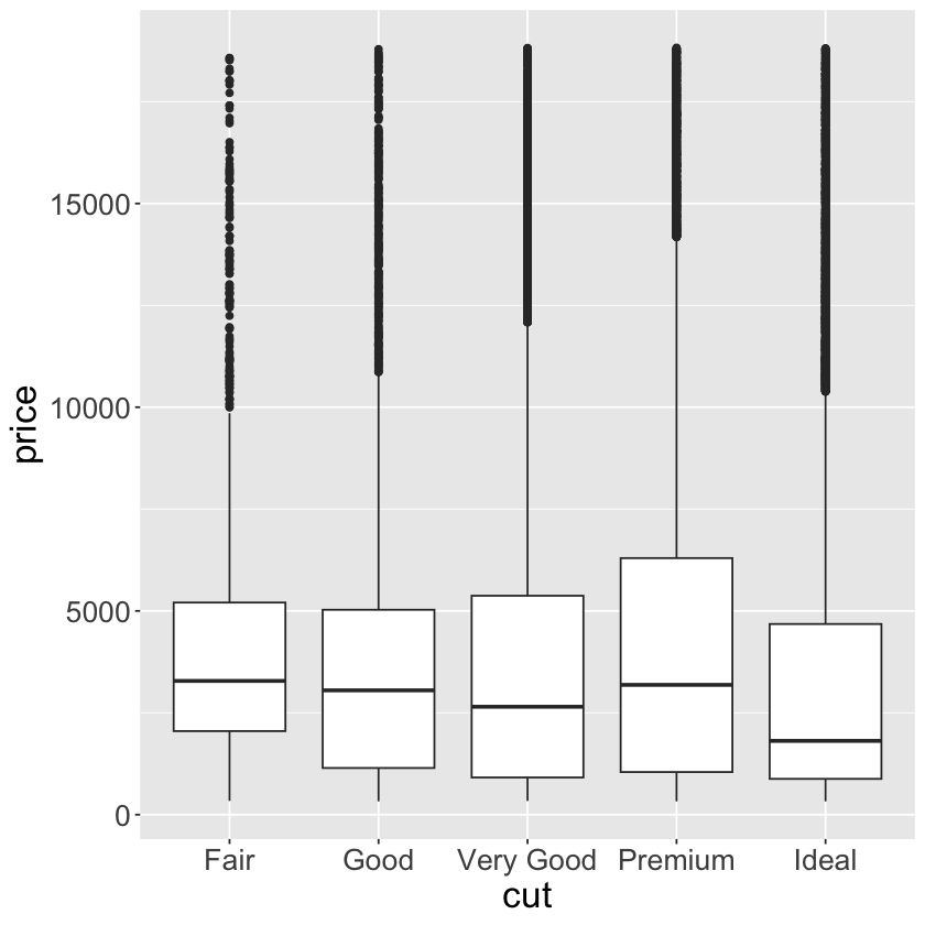
ggplot(data = diamonds, mapping = aes(x = cut, y = price)) +
  geom_boxplot() +
  theme(text = element_text(size = 20))

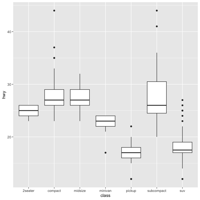
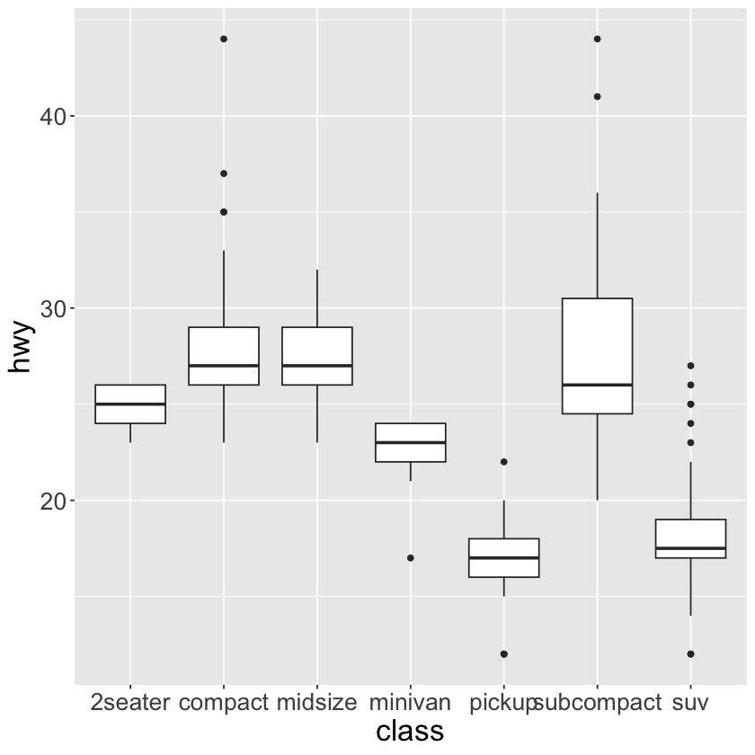
ggplot(data = mpg, mapping = aes(x = class, y = hwy)) +
  geom_boxplot() +
  theme(text = element_text(size = 20))

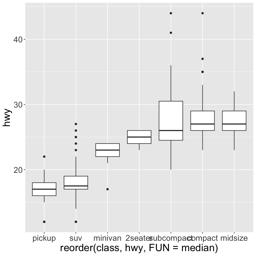
ggplot(data = mpg) +
  geom_boxplot(mapping = aes(x = reorder(class, hwy, FUN = median), y = hwy)) +
  theme(text = element_text(size = 20))

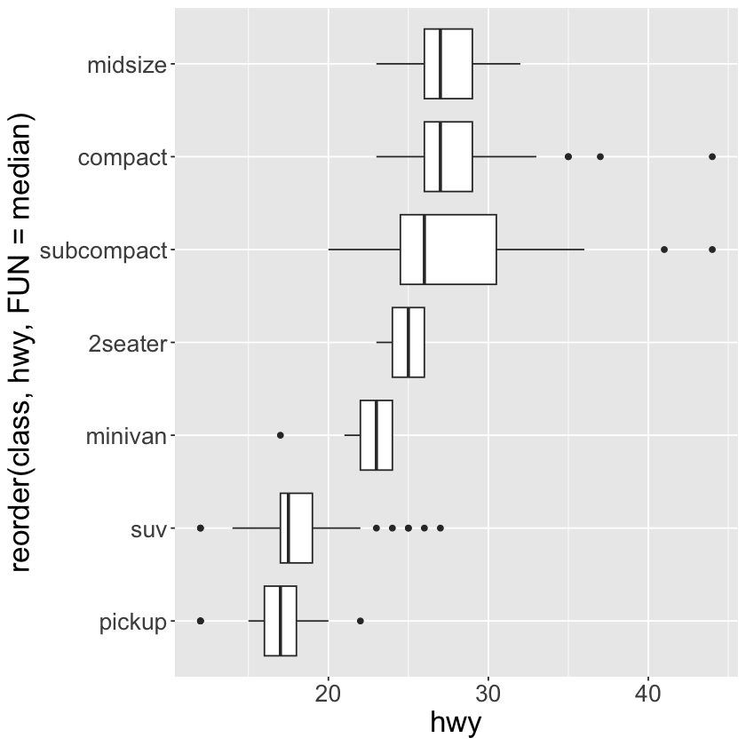
ggplot(data = mpg) +
  geom_boxplot(mapping = aes(x = reorder(class, hwy, FUN = median), y = hwy)) +
  coord_flip() +
  theme(text = element_text(size = 20))

7.5.2 - Two categorical variables

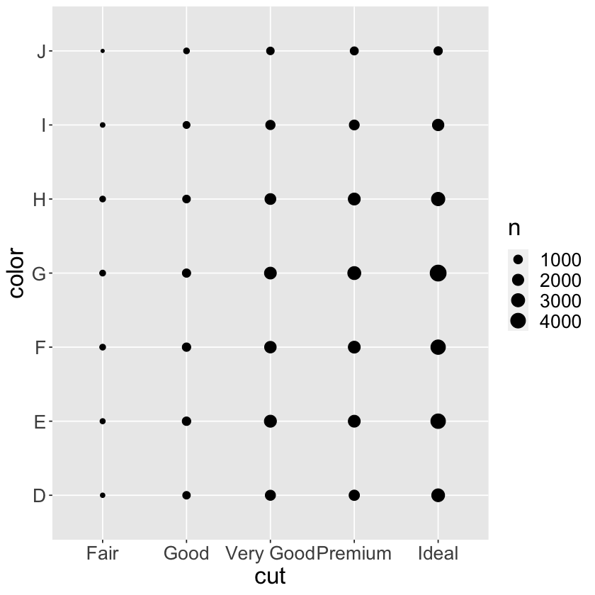
# to visualize the covariation between categorical variables, count the number of observations for each combination
# one way to do this is to rely on the builtin `geom_count()`
# another approach is to compute the count with dplyr, and then visualize with `geom_tile()` and the fill aesthetic
# the size of each circle in the plot displays how many observations occurred at each combination of values
# covariation will appear as a strong correlation between specific x values and specific y values
# if the categorical variables are unordered, use the seriation package to simultaneously reorder the rows and columns in order to more clearly reveal interesting patterns
# for larger plots, try the d3heatmap or heatmaply packages, which create interactive plots

ggplot(data = diamonds) +
  geom_count(mapping = aes(x = cut, y = color)) +
  theme(text = element_text(size = 20))

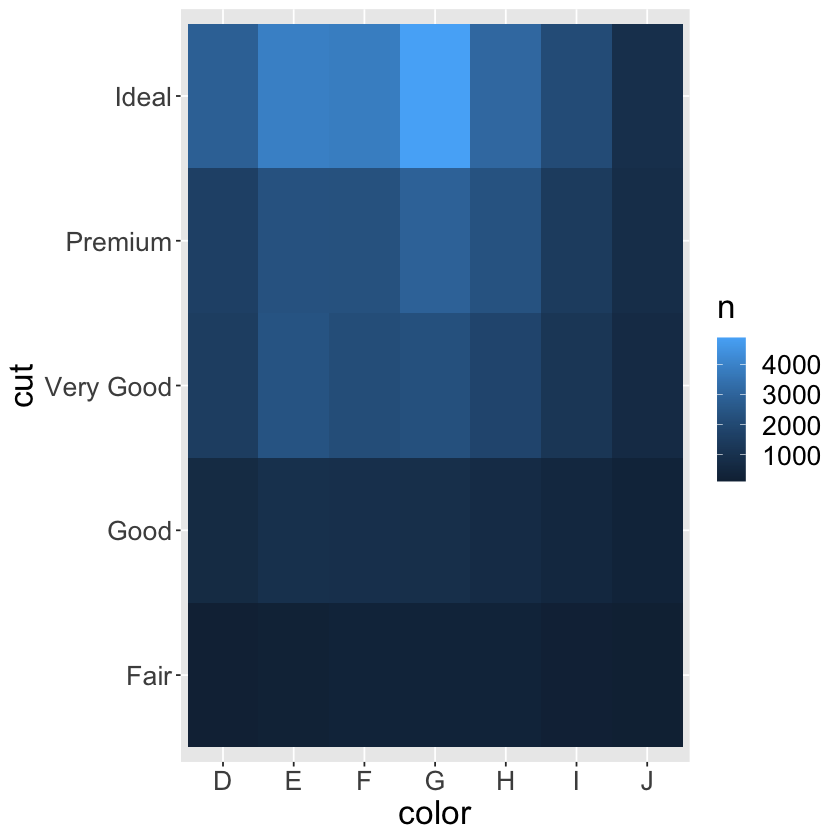
diamonds %>%
  count(color, cut)

diamonds %>%
  count(color, cut) %>%
  ggplot(mapping = aes(x = color, y = cut)) +
    geom_tile(mapping = aes(fill = n)) +
    theme(text = element_text(size = 20))

A tibble: 35 × 3

color	cut	n
<ord>	<ord>	<int>
D	Fair	163
D	Good	662
D	Very Good	1513
D	Premium	1603
D	Ideal	2834
E	Fair	224
E	Good	933
E	Very Good	2400
E	Premium	2337
E	Ideal	3903
F	Fair	312
F	Good	909
F	Very Good	2164
F	Premium	2331
F	Ideal	3826
G	Fair	314
G	Good	871
G	Very Good	2299
G	Premium	2924
G	Ideal	4884
H	Fair	303
H	Good	702
H	Very Good	1824
H	Premium	2360
H	Ideal	3115
I	Fair	175
I	Good	522
I	Very Good	1204
I	Premium	1428
I	Ideal	2093
J	Fair	119
J	Good	307
J	Very Good	678
J	Premium	808
J	Ideal	896

7.5.3 - Two continuous variables

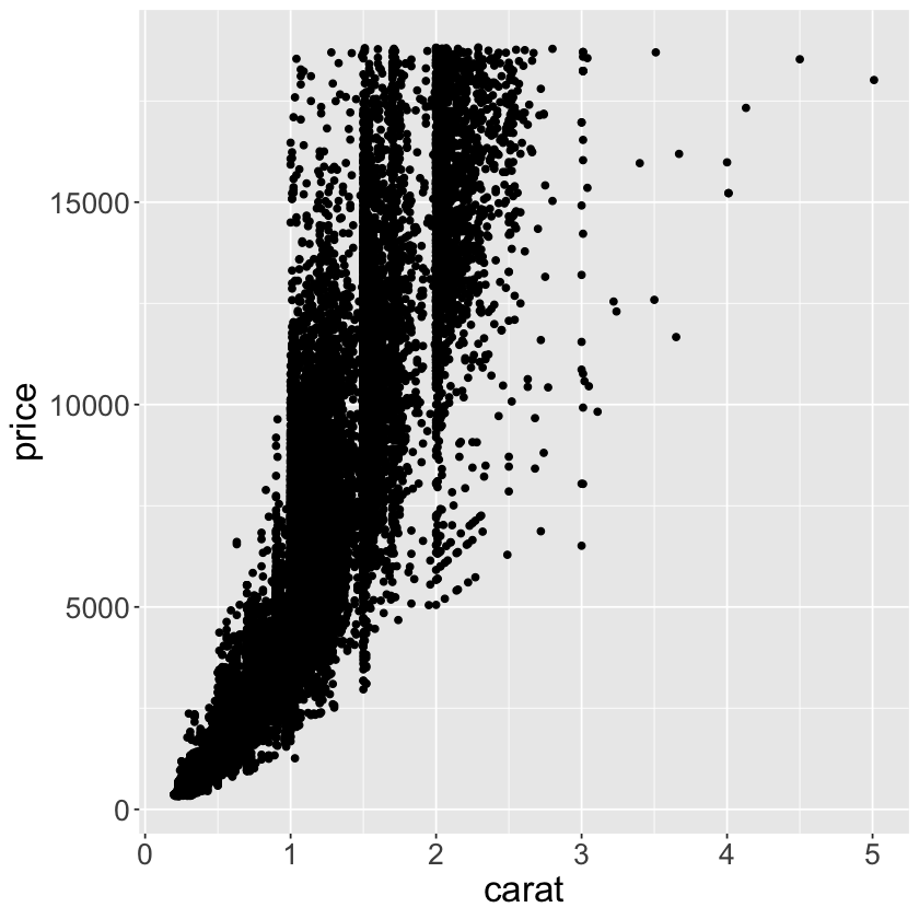
# one way to visualize the covariation between two continuous variables is to draw a scatterplot with `geom_point()`
# covariation can be seen as a pattern in the points
# for example, an expontential relationship between carat size and price of a diamond can be seen

ggplot(data = diamonds) +
  geom_point(mapping = aes(x = carat, y = price)) +
  theme(text = element_text(size = 20))

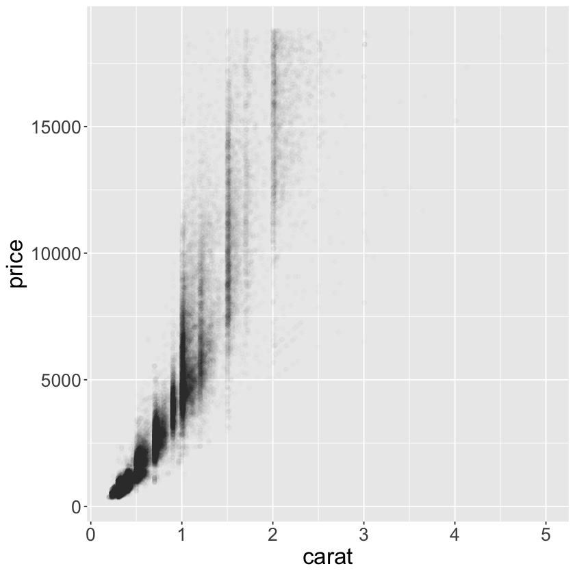
ggplot(data = diamonds) +
  geom_point(mapping = aes(x = carat, y = price), alpha = 1/100) +
  theme(text = element_text(size = 20))

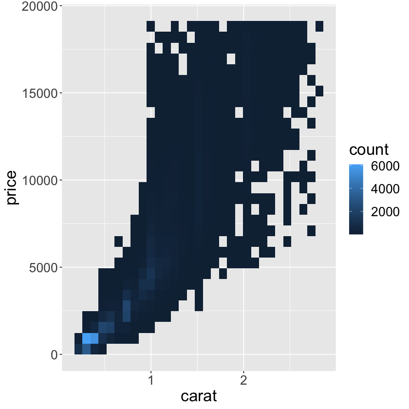
ggplot(data = smaller) +
  geom_bin2d(mapping = aes(x = carat, y = price)) +
  theme(text = element_text(size = 20))

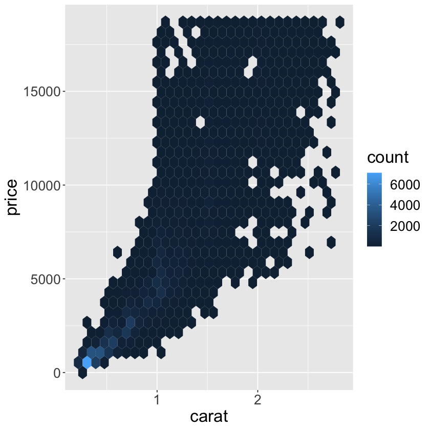
ggplot(data = smaller) +
  geom_hex(mapping = aes(x = carat, y = price)) +
  theme(text = element_text(size = 20))

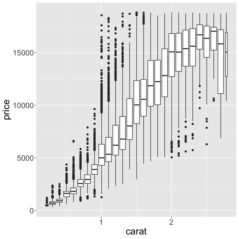
ggplot(data = smaller, mapping = aes(x = carat, y = price)) +
  geom_boxplot(mapping = aes(group = cut_width(x = carat, width = 0.1))) +
  theme(text = element_text(size = 20))

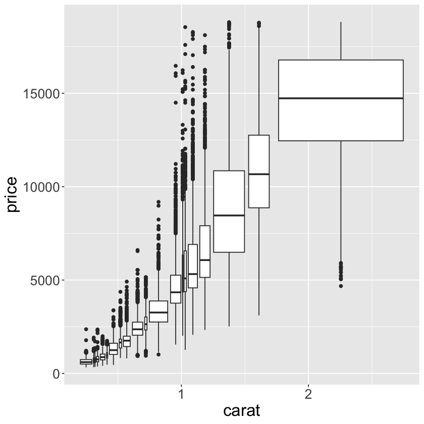
ggplot(data = smaller, mapping = aes(x = carat, y = price)) +
  geom_boxplot(mapping = aes(group = cut_number(x = carat, n = 20))) +
  theme(text = element_text(size = 20))

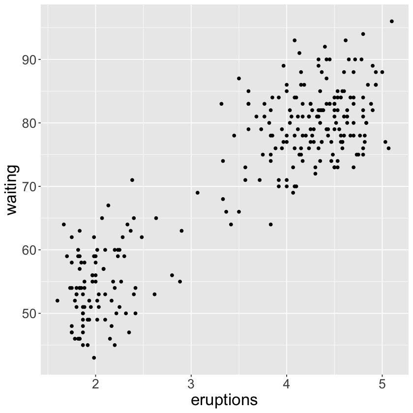
7.6 - Patterns and models

ggplot(data = faithful) +
  geom_point(mapping = aes(x = eruptions, y = waiting)) +
  theme(text = element_text(size = 20))

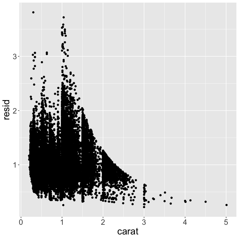
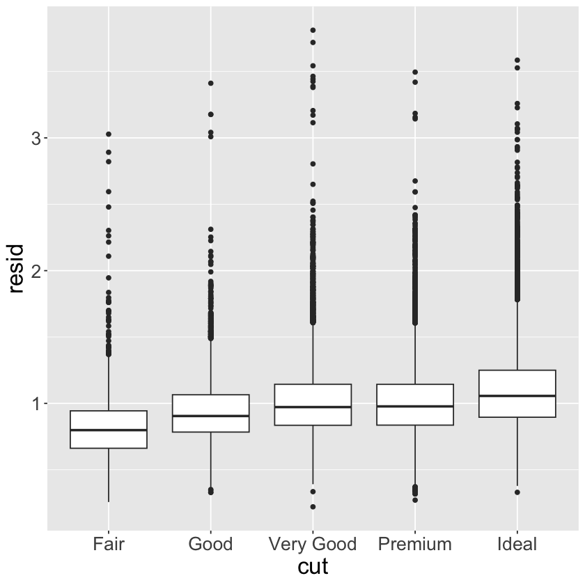
mod <- lm(formula = log(x = price) ~ log(x = carat), data = diamonds)

diamonds2 <-
  diamonds %>%
    add_residuals(model = mod) %>%
    mutate(resid = exp(x = resid))

ggplot(data = diamonds2) +
  geom_point(mapping = aes(x = carat, y = resid)) +
  theme(text = element_text(size = 20))

ggplot(data = diamonds2) +
  geom_boxplot(mapping = aes(x = cut, y = resid)) +
  theme(text = element_text(size = 20))

---

12 - Tidy Data

table1
table2
table3
table4a
table4b

A tibble: 6 × 4

country	year	cases	population
<chr>	<dbl>	<dbl>	<dbl>
Afghanistan	1999	745	19987071
Afghanistan	2000	2666	20595360
Brazil	1999	37737	172006362
Brazil	2000	80488	174504898
China	1999	212258	1272915272
China	2000	213766	1280428583

A tibble: 12 × 4

country	year	type	count
<chr>	<dbl>	<chr>	<dbl>
Afghanistan	1999	cases	745
Afghanistan	1999	population	19987071
Afghanistan	2000	cases	2666
Afghanistan	2000	population	20595360
Brazil	1999	cases	37737
Brazil	1999	population	172006362
Brazil	2000	cases	80488
Brazil	2000	population	174504898
China	1999	cases	212258
China	1999	population	1272915272
China	2000	cases	213766
China	2000	population	1280428583

A tibble: 6 × 3

country	year	rate
<chr>	<dbl>	<chr>
Afghanistan	1999	745/19987071
Afghanistan	2000	2666/20595360
Brazil	1999	37737/172006362
Brazil	2000	80488/174504898
China	1999	212258/1272915272
China	2000	213766/1280428583

A tibble: 3 × 3

country	1999	2000
<chr>	<dbl>	<dbl>
Afghanistan	745	2666
Brazil	37737	80488
China	212258	213766

A tibble: 3 × 3

country	1999	2000
<chr>	<dbl>	<dbl>
Afghanistan	19987071	20595360
Brazil	172006362	174504898
China	1272915272	1280428583

# Compute rate per 10,000
table1 %>%
  mutate(rate = cases / population * 10000)

# Compute cases per year
table1 %>%
  count(year, wt = cases)

# Visualize changes over time
ggplot(table1, aes(year, cases)) +
  geom_line(aes(group = country), color = "grey50") +
  geom_point(aes(color = country))

A tibble: 6 × 5

country	year	cases	population	rate
<chr>	<dbl>	<dbl>	<dbl>	<dbl>
Afghanistan	1999	745	19987071	0.372741
Afghanistan	2000	2666	20595360	1.294466
Brazil	1999	37737	172006362	2.193930
Brazil	2000	80488	174504898	4.612363
China	1999	212258	1272915272	1.667495
China	2000	213766	1280428583	1.669488

A tibble: 2 × 2

year	n
<dbl>	<dbl>
1999	250740
2000	296920

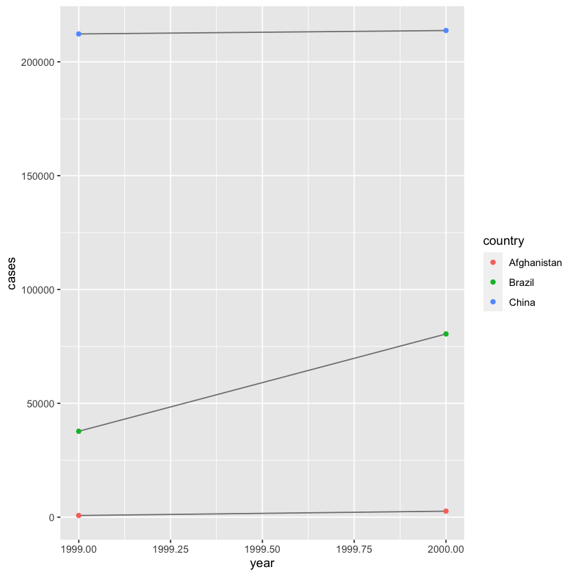
table4a
table4a %>%
  pivot_longer(c(`1999`,`2000`),names_to='year',values_to='cases')
table4b
table4b %>%
  pivot_longer(c(`1999`,`2000`),names_to='year',values_to='population')
tidy4a <- table4a %>%
  pivot_longer(c(`1999`,`2000`),names_to='year',values_to='cases')
tidy4b <- table4b %>%
  pivot_longer(c(`1999`,`2000`),names_to='year',values_to='population')
left_join(tidy4a,tidy4b)

A tibble: 3 × 3

country	1999	2000
<chr>	<dbl>	<dbl>
Afghanistan	745	2666
Brazil	37737	80488
China	212258	213766

A tibble: 6 × 3

country	year	cases
<chr>	<chr>	<dbl>
Afghanistan	1999	745
Afghanistan	2000	2666
Brazil	1999	37737
Brazil	2000	80488
China	1999	212258
China	2000	213766

A tibble: 3 × 3

country	1999	2000
<chr>	<dbl>	<dbl>
Afghanistan	19987071	20595360
Brazil	172006362	174504898
China	1272915272	1280428583

A tibble: 6 × 3

country	year	population
<chr>	<chr>	<dbl>
Afghanistan	1999	19987071
Afghanistan	2000	20595360
Brazil	1999	172006362
Brazil	2000	174504898
China	1999	1272915272
China	2000	1280428583

Joining with `by = join_by(country, year)`

A tibble: 6 × 4

country	year	cases	population
<chr>	<chr>	<dbl>	<dbl>
Afghanistan	1999	745	19987071
Afghanistan	2000	2666	20595360
Brazil	1999	37737	172006362
Brazil	2000	80488	174504898
China	1999	212258	1272915272
China	2000	213766	1280428583

---

13 - Relational data

# tibble `flights` connects to tibble `planes`   via variable  `tailnum`
# tibble `flights` connects to tibble `airlines` via variable  `carrier`
# tibble `flights` connects to tibble `airports` via variables `origin` and `dest`
# tibble `flights` connects to tibble `weather`  via variables `origin`, `year`, `month`, `day`, and `hour`

data(package = 'nycflights13')

# tibble `airlines` looks up the full carrier name from its abbreviated code
head(x = nycflights13::airlines, n = 6)

A tibble: 6 × 2

carrier	name
<chr>	<chr>
9E	Endeavor Air Inc.
AA	American Airlines Inc.
AS	Alaska Airlines Inc.
B6	JetBlue Airways
DL	Delta Air Lines Inc.
EV	ExpressJet Airlines Inc.

# tibble `airports` gives info about each airport each of which is identified by the faa airport code
head(x = nycflights13::airports, n = 6)

A tibble: 6 × 8

faa	name	lat	lon	alt	tz	dst	tzone
<chr>	<chr>	<dbl>	<dbl>	<dbl>	<dbl>	<chr>	<chr>
04G	Lansdowne Airport	41.13047	-80.61958	1044	-5	A	America/New_York
06A	Moton Field Municipal Airport	32.46057	-85.68003	264	-6	A	America/Chicago
06C	Schaumburg Regional	41.98934	-88.10124	801	-6	A	America/Chicago
06N	Randall Airport	41.43191	-74.39156	523	-5	A	America/New_York
09J	Jekyll Island Airport	31.07447	-81.42778	11	-5	A	America/New_York
0A9	Elizabethton Municipal Airport	36.37122	-82.17342	1593	-5	A	America/New_York

# tibble `flights`
#   foreign key - tailnum

head(x = nycflights13::flights, n = 6)

# not quite the primary key
flights %>%
  count(year, month, day, flight, tailnum) %>%
    filter(n > 1)

A tibble: 6 × 19

year	month	day	dep_time	sched_dep_time	dep_delay	arr_time	sched_arr_time	arr_delay	carrier	flight	tailnum	origin	dest	air_time	distance	hour	minute	time_hour
<int>	<int>	<int>	<int>	<int>	<dbl>	<int>	<int>	<dbl>	<chr>	<int>	<chr>	<chr>	<chr>	<dbl>	<dbl>	<dbl>	<dbl>	<dttm>
2013	1	1	517	515	2	830	819	11	UA	1545	N14228	EWR	IAH	227	1400	5	15	2013-01-01 05:00:00
2013	1	1	533	529	4	850	830	20	UA	1714	N24211	LGA	IAH	227	1416	5	29	2013-01-01 05:00:00
2013	1	1	542	540	2	923	850	33	AA	1141	N619AA	JFK	MIA	160	1089	5	40	2013-01-01 05:00:00
2013	1	1	544	545	-1	1004	1022	-18	B6	725	N804JB	JFK	BQN	183	1576	5	45	2013-01-01 05:00:00
2013	1	1	554	600	-6	812	837	-25	DL	461	N668DN	LGA	ATL	116	762	6	0	2013-01-01 06:00:00
2013	1	1	554	558	-4	740	728	12	UA	1696	N39463	EWR	ORD	150	719	5	58	2013-01-01 05:00:00

A tibble: 11 × 6

year	month	day	flight	tailnum	n
<int>	<int>	<int>	<int>	<chr>	<int>
2013	2	9	303	NA	2
2013	2	9	655	NA	2
2013	2	9	1623	NA	2
2013	6	8	2269	N487WN	2
2013	6	15	2269	N230WN	2
2013	6	22	2269	N440LV	2
2013	6	29	2269	N707SA	2
2013	7	6	2269	N259WN	2
2013	8	3	2269	N446WN	2
2013	8	10	2269	N478WN	2
2013	12	15	398	NA	2

# tibble `planes` gives info about planes each of which is identified by its tailnum
#   primary key - variable `tailnum`

head(x = nycflights13::planes, n = 6)

planes %>%
  count(tailnum) %>%
    filter(n > 1)

A tibble: 6 × 9

tailnum	year	type	manufacturer	model	engines	seats	speed	engine
<chr>	<int>	<chr>	<chr>	<chr>	<int>	<int>	<int>	<chr>
N10156	2004	Fixed wing multi engine	EMBRAER	EMB-145XR	2	55	NA	Turbo-fan
N102UW	1998	Fixed wing multi engine	AIRBUS INDUSTRIE	A320-214	2	182	NA	Turbo-fan
N103US	1999	Fixed wing multi engine	AIRBUS INDUSTRIE	A320-214	2	182	NA	Turbo-fan
N104UW	1999	Fixed wing multi engine	AIRBUS INDUSTRIE	A320-214	2	182	NA	Turbo-fan
N10575	2002	Fixed wing multi engine	EMBRAER	EMB-145LR	2	55	NA	Turbo-fan
N105UW	1999	Fixed wing multi engine	AIRBUS INDUSTRIE	A320-214	2	182	NA	Turbo-fan

A tibble: 0 × 2

tailnum	n
<chr>	<int>

# tibble `weather` gives the weather at each NYC airport for each hour
#   primary key? - variables `year`, `month`, `day`, `hour`, `origin`

head(x = nycflights13::weather, n = 6)

# not quite the primary key
weather %>%
  count(year, month, day, hour, origin) %>%
    filter(n > 1)

A tibble: 6 × 15

origin	year	month	day	hour	temp	dewp	humid	wind_dir	wind_speed	wind_gust	precip	pressure	visib	time_hour
<chr>	<int>	<int>	<int>	<int>	<dbl>	<dbl>	<dbl>	<dbl>	<dbl>	<dbl>	<dbl>	<dbl>	<dbl>	<dttm>
EWR	2013	1	1	1	39.02	26.06	59.37	270	10.35702	NA	0	1012.0	10	2013-01-01 01:00:00
EWR	2013	1	1	2	39.02	26.96	61.63	250	8.05546	NA	0	1012.3	10	2013-01-01 02:00:00
EWR	2013	1	1	3	39.02	28.04	64.43	240	11.50780	NA	0	1012.5	10	2013-01-01 03:00:00
EWR	2013	1	1	4	39.92	28.04	62.21	250	12.65858	NA	0	1012.2	10	2013-01-01 04:00:00
EWR	2013	1	1	5	39.02	28.04	64.43	260	12.65858	NA	0	1011.9	10	2013-01-01 05:00:00
EWR	2013	1	1	6	37.94	28.04	67.21	240	11.50780	NA	0	1012.4	10	2013-01-01 06:00:00

A tibble: 3 × 6

year	month	day	hour	origin	n
<int>	<int>	<int>	<int>	<chr>	<int>
2013	11	3	1	EWR	2
2013	11	3	1	JFK	2
2013	11	3	1	LGA	2

flights2 <-
  flights %>%
    select(year:day, hour, origin, dest, tailnum, carrier)
head(x = flights2, n = 6)

A tibble: 6 × 8

year	month	day	hour	origin	dest	tailnum	carrier
<int>	<int>	<int>	<dbl>	<chr>	<chr>	<chr>	<chr>
2013	1	1	5	EWR	IAH	N14228	UA
2013	1	1	5	LGA	IAH	N24211	UA
2013	1	1	5	JFK	MIA	N619AA	AA
2013	1	1	5	JFK	BQN	N804JB	B6
2013	1	1	6	LGA	ATL	N668DN	DL
2013	1	1	5	EWR	ORD	N39463	UA

flights2 %>%
  select(-origin, -dest) %>%
    left_join(y = airlines, by = 'carrier') %>%
      head(n = 6)

A tibble: 6 × 7

year	month	day	hour	tailnum	carrier	name
<int>	<int>	<int>	<dbl>	<chr>	<chr>	<chr>
2013	1	1	5	N14228	UA	United Air Lines Inc.
2013	1	1	5	N24211	UA	United Air Lines Inc.
2013	1	1	5	N619AA	AA	American Airlines Inc.
2013	1	1	5	N804JB	B6	JetBlue Airways
2013	1	1	6	N668DN	DL	Delta Air Lines Inc.
2013	1	1	5	N39463	UA	United Air Lines Inc.

flights2 %>%
  select(-origin, -dest) %>%
    mutate(
      name = airlines$name[match(carrier, airlines$carrier)]
    ) %>%
      head(n = 6)

A tibble: 6 × 7

year	month	day	hour	tailnum	carrier	name
<int>	<int>	<int>	<dbl>	<chr>	<chr>	<chr>
2013	1	1	5	N14228	UA	United Air Lines Inc.
2013	1	1	5	N24211	UA	United Air Lines Inc.
2013	1	1	5	N619AA	AA	American Airlines Inc.
2013	1	1	5	N804JB	B6	JetBlue Airways
2013	1	1	6	N668DN	DL	Delta Air Lines Inc.
2013	1	1	5	N39463	UA	United Air Lines Inc.

x <- tribble(
  ~key, ~val_x,
     1,   'x1',
     2,   'x2',
     3,   'x3'
)

y <- tribble(
  ~key, ~val_y,
     1,   'y1',
     2,   'y2',
     4,   'y3'
)

inner_join(x = x, y = y, by = 'key')

base::merge(x = x, y = y)

A tibble: 2 × 3

key	val_x	val_y
<dbl>	<chr>	<chr>
1	x1	y1
2	x2	y2

A data.frame: 2 × 3

key	val_x	val_y
<dbl>	<chr>	<chr>
1	x1	y1
2	x2	y2

# ONE TABLE HAS DUPLICATE KEYS
#   this is useful when you want to add in additional info (there is typically a one-to-many relationship)

x <- tribble(
  ~key, ~val_x,
     1,   'x1',
     2,   'x2',
     2,   'x3',
     1,   'x4'
)

y <- tribble(
  ~key, ~val_y,
     1,   'y1',
     2,   'y2'
)

left_join(x = x, y = y, by = 'key')

base::merge(x = x, y = y)

A tibble: 4 × 3

key	val_x	val_y
<dbl>	<chr>	<chr>
1	x1	y1
2	x2	y2
2	x3	y2
1	x4	y1

A data.frame: 4 × 3

key	val_x	val_y
<dbl>	<chr>	<chr>
1	x1	y1
1	x4	y1
2	x2	y2
2	x3	y2

# BOTH TABLES HAVE DUPLICATE KEYS
#   this is usually an error because in neither table do the keys uniquely identify an observation
#   when you join duplicated keys you get all possible combinations, the Cartesian product

x <- tribble(
  ~key, ~val_x,
     1,   'x1',
     2,   'x2',
     2,   'x3',
     3,   'x4'
)

y <- tribble(
  ~key, ~val_y,
     1,   'y1',
     2,   'y2',
     2,   'y3',
     3,   'y4'
)

left_join(x = x, y = y, by = 'key')

base::merge(x = x, y = y)

Warning message in left_join(x = x, y = y, by = "key"):
“Detected an unexpected many-to-many relationship between `x` and `y`.
ℹ Row 2 of `x` matches multiple rows in `y`.
ℹ Row 2 of `y` matches multiple rows in `x`.
ℹ If a many-to-many relationship is expected, set `relationship = "many-to-many"` to silence this warning.”

A tibble: 6 × 3

key	val_x	val_y
<dbl>	<chr>	<chr>
1	x1	y1
2	x2	y2
2	x2	y3
2	x3	y2
2	x3	y3
3	x4	y4

A data.frame: 6 × 3

key	val_x	val_y
<dbl>	<chr>	<chr>
1	x1	y1
2	x2	y2
2	x2	y3
2	x3	y2
2	x3	y3
3	x4	y4

# NATURAL JOIN
#   by = c('year', 'month', 'day', 'hour', 'origin')

flights2 %>%
  left_join(y = weather) %>%
    head()

Joining with `by = join_by(year, month, day, hour, origin)`

A tibble: 6 × 18

year	month	day	hour	origin	dest	tailnum	carrier	temp	dewp	humid	wind_dir	wind_speed	wind_gust	precip	pressure	visib	time_hour
<int>	<int>	<int>	<dbl>	<chr>	<chr>	<chr>	<chr>	<dbl>	<dbl>	<dbl>	<dbl>	<dbl>	<dbl>	<dbl>	<dbl>	<dbl>	<dttm>
2013	1	1	5	EWR	IAH	N14228	UA	39.02	28.04	64.43	260	12.65858	NA	0	1011.9	10	2013-01-01 05:00:00
2013	1	1	5	LGA	IAH	N24211	UA	39.92	24.98	54.81	250	14.96014	21.86482	0	1011.4	10	2013-01-01 05:00:00
2013	1	1	5	JFK	MIA	N619AA	AA	39.02	26.96	61.63	260	14.96014	NA	0	1012.1	10	2013-01-01 05:00:00
2013	1	1	5	JFK	BQN	N804JB	B6	39.02	26.96	61.63	260	14.96014	NA	0	1012.1	10	2013-01-01 05:00:00
2013	1	1	6	LGA	ATL	N668DN	DL	39.92	24.98	54.81	260	16.11092	23.01560	0	1011.7	10	2013-01-01 06:00:00
2013	1	1	5	EWR	ORD	N39463	UA	39.02	28.04	64.43	260	12.65858	NA	0	1011.9	10	2013-01-01 05:00:00

flights2 %>%
  left_join(y = planes, by = 'tailnum') %>%
    head()

A tibble: 6 × 16

year.x	month	day	hour	origin	dest	tailnum	carrier	year.y	type	manufacturer	model	engines	seats	speed	engine
<int>	<int>	<int>	<dbl>	<chr>	<chr>	<chr>	<chr>	<int>	<chr>	<chr>	<chr>	<int>	<int>	<int>	<chr>
2013	1	1	5	EWR	IAH	N14228	UA	1999	Fixed wing multi engine	BOEING	737-824	2	149	NA	Turbo-fan
2013	1	1	5	LGA	IAH	N24211	UA	1998	Fixed wing multi engine	BOEING	737-824	2	149	NA	Turbo-fan
2013	1	1	5	JFK	MIA	N619AA	AA	1990	Fixed wing multi engine	BOEING	757-223	2	178	NA	Turbo-fan
2013	1	1	5	JFK	BQN	N804JB	B6	2012	Fixed wing multi engine	AIRBUS	A320-232	2	200	NA	Turbo-fan
2013	1	1	6	LGA	ATL	N668DN	DL	1991	Fixed wing multi engine	BOEING	757-232	2	178	NA	Turbo-fan
2013	1	1	5	EWR	ORD	N39463	UA	2012	Fixed wing multi engine	BOEING	737-924ER	2	191	NA	Turbo-fan

flights2 %>%
  left_join(y = airports, by = c('dest' = 'faa')) %>%
    head()

A tibble: 6 × 15

year	month	day	hour	origin	dest	tailnum	carrier	name	lat	lon	alt	tz	dst	tzone
<int>	<int>	<int>	<dbl>	<chr>	<chr>	<chr>	<chr>	<chr>	<dbl>	<dbl>	<dbl>	<dbl>	<chr>	<chr>
2013	1	1	5	EWR	IAH	N14228	UA	George Bush Intercontinental	29.98443	-95.34144	97	-6	A	America/Chicago
2013	1	1	5	LGA	IAH	N24211	UA	George Bush Intercontinental	29.98443	-95.34144	97	-6	A	America/Chicago
2013	1	1	5	JFK	MIA	N619AA	AA	Miami Intl	25.79325	-80.29056	8	-5	A	America/New_York
2013	1	1	5	JFK	BQN	N804JB	B6	NA	NA	NA	NA	NA	NA	NA
2013	1	1	6	LGA	ATL	N668DN	DL	Hartsfield Jackson Atlanta Intl	33.63672	-84.42807	1026	-5	A	America/New_York
2013	1	1	5	EWR	ORD	N39463	UA	Chicago Ohare Intl	41.97860	-87.90484	668	-6	A	America/Chicago

flights2 %>%
  left_join(y = airports, by = c('origin' = 'faa')) %>%
    head()

A tibble: 6 × 15

year	month	day	hour	origin	dest	tailnum	carrier	name	lat	lon	alt	tz	dst	tzone
<int>	<int>	<int>	<dbl>	<chr>	<chr>	<chr>	<chr>	<chr>	<dbl>	<dbl>	<dbl>	<dbl>	<chr>	<chr>
2013	1	1	5	EWR	IAH	N14228	UA	Newark Liberty Intl	40.69250	-74.16867	18	-5	A	America/New_York
2013	1	1	5	LGA	IAH	N24211	UA	La Guardia	40.77725	-73.87261	22	-5	A	America/New_York
2013	1	1	5	JFK	MIA	N619AA	AA	John F Kennedy Intl	40.63975	-73.77893	13	-5	A	America/New_York
2013	1	1	5	JFK	BQN	N804JB	B6	John F Kennedy Intl	40.63975	-73.77893	13	-5	A	America/New_York
2013	1	1	6	LGA	ATL	N668DN	DL	La Guardia	40.77725	-73.87261	22	-5	A	America/New_York
2013	1	1	5	EWR	ORD	N39463	UA	Newark Liberty Intl	40.69250	-74.16867	18	-5	A	America/New_York

options(repr.plot.width=20, repr.plot.height=10)

airports %>%
  semi_join(y = flights, by = c('faa' = 'dest')) %>%
    ggplot(mapping = aes(x = lon, y = lat, size = )) +
      borders('state') +
      geom_point() +
      coord_quickmap() +
      theme(
        text=element_text(size=20)
      )

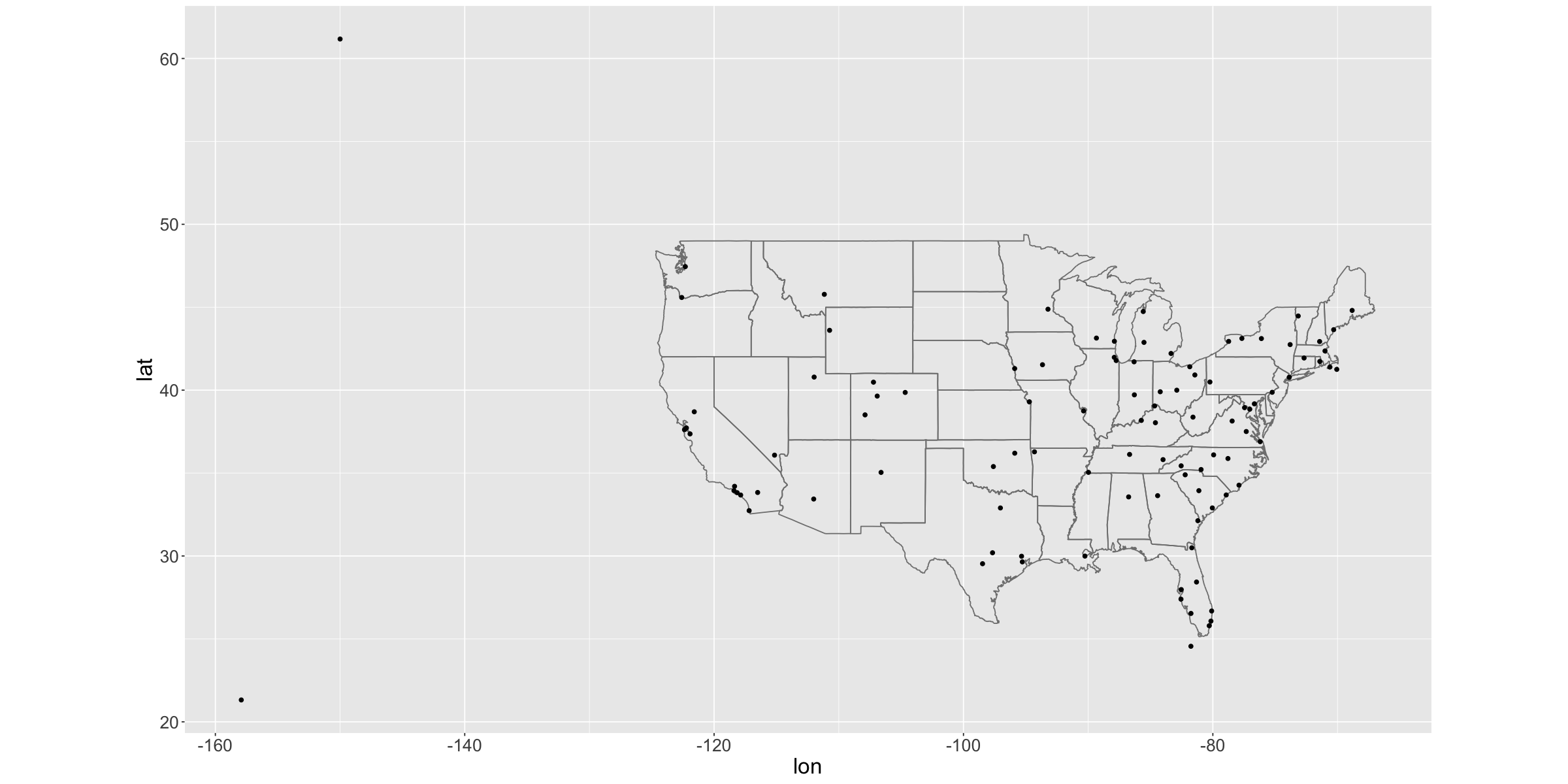
Filtering Joins

Semi Join

x <- tribble(
  ~key, ~val_x,
     1,   'x1',
     2,   'x2',
     3,   'x3'
)

y <- tribble(
  ~key, ~val_y,
     1,   'y1',
     2,   'y2',
     4,   'y3'
)

semi_join(x = x, y = y)

Joining with `by = join_by(key)`

A tibble: 2 × 2

key	val_x
<dbl>	<chr>
1	x1
2	x2

x <- tribble(
  ~key, ~val_x,
     1,   'x1',
     2,   'x2',
     2,   'x3',
     3,   'x4'
)

y <- tribble(
  ~key, ~val_y,
     1,   'y1',
     2,   'y2',
     2,   'y3',
     3,   'y4'
)

semi_join(x = x, y = y)

Joining with `by = join_by(key)`

A tibble: 4 × 2

key	val_x
<dbl>	<chr>
1	x1
2	x2
2	x3
3	x4

top_dest <-
  flights %>%
    count(dest, sort = TRUE) %>%
      head(n = 10)
top_dest

flights %>%
  filter(dest %in% top_dest$dest) %>%
    head()

flights %>%
  semi_join(y = top_dest) %>%
    head()

A tibble: 10 × 2

dest	n
<chr>	<int>
ORD	17283
ATL	17215
LAX	16174
BOS	15508
MCO	14082
CLT	14064
SFO	13331
FLL	12055
MIA	11728
DCA	9705

A tibble: 6 × 19

year	month	day	dep_time	sched_dep_time	dep_delay	arr_time	sched_arr_time	arr_delay	carrier	flight	tailnum	origin	dest	air_time	distance	hour	minute	time_hour
<int>	<int>	<int>	<int>	<int>	<dbl>	<int>	<int>	<dbl>	<chr>	<int>	<chr>	<chr>	<chr>	<dbl>	<dbl>	<dbl>	<dbl>	<dttm>
2013	1	1	542	540	2	923	850	33	AA	1141	N619AA	JFK	MIA	160	1089	5	40	2013-01-01 05:00:00
2013	1	1	554	600	-6	812	837	-25	DL	461	N668DN	LGA	ATL	116	762	6	0	2013-01-01 06:00:00
2013	1	1	554	558	-4	740	728	12	UA	1696	N39463	EWR	ORD	150	719	5	58	2013-01-01 05:00:00
2013	1	1	555	600	-5	913	854	19	B6	507	N516JB	EWR	FLL	158	1065	6	0	2013-01-01 06:00:00
2013	1	1	557	600	-3	838	846	-8	B6	79	N593JB	JFK	MCO	140	944	6	0	2013-01-01 06:00:00
2013	1	1	558	600	-2	753	745	8	AA	301	N3ALAA	LGA	ORD	138	733	6	0	2013-01-01 06:00:00

Joining with `by = join_by(dest)`

A tibble: 6 × 19

year	month	day	dep_time	sched_dep_time	dep_delay	arr_time	sched_arr_time	arr_delay	carrier	flight	tailnum	origin	dest	air_time	distance	hour	minute	time_hour
<int>	<int>	<int>	<int>	<int>	<dbl>	<int>	<int>	<dbl>	<chr>	<int>	<chr>	<chr>	<chr>	<dbl>	<dbl>	<dbl>	<dbl>	<dttm>
2013	1	1	542	540	2	923	850	33	AA	1141	N619AA	JFK	MIA	160	1089	5	40	2013-01-01 05:00:00
2013	1	1	554	600	-6	812	837	-25	DL	461	N668DN	LGA	ATL	116	762	6	0	2013-01-01 06:00:00
2013	1	1	554	558	-4	740	728	12	UA	1696	N39463	EWR	ORD	150	719	5	58	2013-01-01 05:00:00
2013	1	1	555	600	-5	913	854	19	B6	507	N516JB	EWR	FLL	158	1065	6	0	2013-01-01 06:00:00
2013	1	1	557	600	-3	838	846	-8	B6	79	N593JB	JFK	MCO	140	944	6	0	2013-01-01 06:00:00
2013	1	1	558	600	-2	753	745	8	AA	301	N3ALAA	LGA	ORD	138	733	6	0	2013-01-01 06:00:00

Anti Join

x <- tribble(
  ~key, ~val_x,
     1,   'x1',
     2,   'x2',
     3,   'x3'
)

y <- tribble(
  ~key, ~val_y,
     1,   'y1',
     2,   'y2',
     4,   'y3'
)

anti_join(x = x, y = y)

Joining with `by = join_by(key)`

A tibble: 1 × 2

key	val_x
<dbl>	<chr>
3	x3

x <- tribble(
  ~key, ~val_x,
     1,   'x1',
     2,   'x2',
     2,   'x3',
     3,   'x4'
)

y <- tribble(
  ~key, ~val_y,
     1,   'y1',
     2,   'y2',
     2,   'y3',
     3,   'y4'
)

anti_join(x = x, y = y)

Joining with `by = join_by(key)`

A tibble: 0 × 2

key	val_x
<dbl>	<chr>

# anti joins are useful for diagnosing join mismatches
# for example, you might be interested to know that there are many `flights` that don't have a match in `planes`

flights %>%
  anti_join(y = planes, by = 'tailnum') %>%
    count(tailnum, sort = TRUE) %>%
      head()

A tibble: 6 × 2

tailnum	n
<chr>	<int>
NA	2512
N725MQ	575
N722MQ	513
N723MQ	507
N713MQ	483
N735MQ	396

13.7 - Set operations

df1 <- tribble(
  ~x, ~y,
   1,  1,
   2,  1
)

df2 <- tribble(
  ~x, ~y,
   1,  1,
   1,  2
)

intersect(x = df1, y = df2)

union(x = df1, y = df2)

setdiff(x = df1, y = df2)

setdiff(x = df2, y = df1)

A tibble: 1 × 2

x	y
<dbl>	<dbl>
1	1

A tibble: 3 × 2

x	y
<dbl>	<dbl>
1	1
2	1
1	2

A tibble: 1 × 2

x	y
<dbl>	<dbl>
2	1

A tibble: 1 × 2

x	y
<dbl>	<dbl>
1	2

---

14 - Strings

string1      <- "This is a string"
string2      <- 'If I want to include a "quote" inside a string, I use single quotes'
double_quote <- "\"" # or '"'
single_quote <- '\'' # or "'"

# the printed representation of a string is not the same as the string itself
x <- c("\"", "\\")
x
writeLines(x)

1. '"'
2. '\\'

"
\

?'"'

x <- "\u00b5"
x

c('one', 'two', 'three')

'µ'

1. 'one'
2. 'two'
3. 'three'

str_length(c('a', 'R for data science', NA))

1. 1
2. 18
3. <NA>

str_c('x', 'y', 'z')

'xyz'

x <- c('abc', NA)

str_c('|-', x, '-|')

str_c('|-', str_replace_na(x), '-|')

1. '|-abc-|'
2. NA

1. '|-abc-|'
2. '|-NA-|'

str_c('prefix-', c('a', 'b', 'c'), '-suffix')

1. 'prefix-a-suffix'
2. 'prefix-b-suffix'
3. 'prefix-c-suffix'

name        <- 'Hadley'
time_of_day <- 'morning'
birthday    <- FALSE

str_c('Good ', time_of_day, ' ', name, if (birthday) ' and HAPPY BIRTHDAY', '.')

'Good morning Hadley.'

str_c(c('x', 'y', 'z'), collapse = ', ')

'x, y, z'

x <- c('Apple', 'Banana', 'Pear')

str_sub(x,  1,  3)
str_sub(x, -3, -1)
str_sub(x,  1, 10)

1. 'App'
2. 'Ban'
3. 'Pea'

1. 'ple'
2. 'ana'
3. 'ear'

1. 'Apple'
2. 'Banana'
3. 'Pear'

str_sub(x, 1, 1) <- str_to_lower(str_sub(x, 1, 1))

x

1. 'apple'
2. 'banana'
3. 'pear'

str_to_upper(c('i', 'ı'))
str_to_upper(c('i', 'ı'), locale = 'tr')

1. 'I'
2. 'I'

1. 'İ'
2. 'I'

x <- c('apple', 'eggplant', 'banana')

str_sort(x, locale = 'en')  # English
str_sort(x, locale = 'haw') # Hawaiian

1. 'apple'
2. 'banana'
3. 'eggplant'

1. 'apple'
2. 'eggplant'
3. 'banana'

x <- c('apple', 'banana', 'pear')

str_view(x, 'an')

[2] │ b<an><an>a

str_view(x, '.a.')

[2] │ <ban>ana
[3] │ p<ear>

dot <- '\\.'

dot

writeLines(dot)

'\\.'

\.

str_view(c('abc', 'a.c', 'bef'), 'a\\.c')

[2] │ <a.c>

x <- 'a\\b'

x

writeLines(x)

str_view(x, '\\\\')

'a\\b'

a\b

[1] │ a<\>b

x <- 

Error in parse(text = x, srcfile = src): <text>:2:0: unexpected end of input
1: x <- 
   ^
Traceback:

---

16 - Dates and times

today()

2023-06-19

now()

[1] "2023-06-19 21:40:12 EDT"

lubridate::ymd('2017-01-31')
lubridate::mdy('January 31st, 2017')
lubridate::dmy('31-Jan-2017')
lubridate::ymd(20170131)
lubridate::ymd_hms('2017-01-31 20:11:59')
lubridate::mdy_hm('01/31/2017 08:01')
lubridate::ymd(20170131, tz = 'UTC')

2017-01-31

2017-01-31

2017-01-31

2017-01-31

[1] "2017-01-31 20:11:59 UTC"

[1] "2017-01-31 08:01:00 UTC"

[1] "2017-01-31 UTC"

---

19 - Functions

df <- tibble::tibble(
  a = rnorm(10),
  b = rnorm(10),
  c = rnorm(10),
  d = rnorm(10),
)
df$a <- (df$a - min(df$a, na.rm = TRUE)) / (max(df$a, na.rm = TRUE) - min(df$a, na.rm = TRUE))
df$b <- (df$b - min(df$b, na.rm = TRUE)) / (max(df$d, na.rm = TRUE) - min(df$b, na.rm = TRUE))
df$c <- (df$c - min(df$c, na.rm = TRUE)) / (max(df$c, na.rm = TRUE) - min(df$c, na.rm = TRUE))
df$d <- (df$d - min(df$d, na.rm = TRUE)) / (max(df$d, na.rm = TRUE) - min(df$d, na.rm = TRUE))
df

A tibble: 10 × 4

a	b	c	d
<dbl>	<dbl>	<dbl>	<dbl>
0.2603453	0.0000000	0.52291366	0.17190835
0.4428665	0.3911715	0.00000000	0.34864602
0.7679751	0.2958880	0.61301233	0.00000000
0.0000000	0.3256557	0.03846392	1.00000000
0.9597766	0.3409009	0.30398213	0.38970973
0.7516023	0.2671197	1.00000000	0.14085417
1.0000000	0.4352529	0.35195509	0.08903446
0.3199440	0.5370480	0.57422199	0.77900010
0.7130083	0.0714432	0.37854517	0.07351166
0.1629208	0.1235444	0.53272103	0.50560502

rescale01 <- function (x) {
  rng <- range(x, na.rm = TRUE)
  (x - rng[1]) / (rng[2] - rng[1])
}

rescale01(c(0, 5, 10))
rescale01(c(-10, 0, 10))
rescale01(c(1, 2, 3, NA, 5))

1. 0
2. 0.5
3. 1

1. 0
2. 0.5
3. 1

1. 0
2. 0.25
3. 0.5
4. <NA>
5. 1

df <- tibble::tibble(
  a = rnorm(10),
  b = rnorm(10),
  c = rnorm(10),
  d = rnorm(10),
)
df$a <- rescale01(df$a)
df$b <- rescale01(df$b)
df$c <- rescale01(df$c)
df$d <- rescale01(df$d)
df

A tibble: 10 × 4

a	b	c	d
<dbl>	<dbl>	<dbl>	<dbl>
0.5620421	0.4772677	0.00000000	0.2779846
0.0000000	0.1481486	0.20080052	0.2611846
0.3120153	0.8396613	0.04548743	0.4313317
0.5319523	0.6228401	0.47050875	0.9074133
0.4530802	0.3482687	0.33315823	0.1256405
0.4333381	1.0000000	0.33140720	0.5639065
0.4721171	0.5706066	0.14447456	0.7455952
0.1415588	0.0000000	0.15490717	1.0000000
1.0000000	0.3948759	1.00000000	0.0000000
0.3231058	0.6069666	0.73818349	0.9683428

x <- c(1:10, Inf)

rescale01(x)

1. 0
2. 0
3. 0
4. 0
5. 0
6. 0
7. 0
8. 0
9. 0
10. 0
11. NaN

rescale01 <- function (x) {
  rng <- range(x, na.rm = TRUE, finite = TRUE)
  (x - rng[1]) / (rng[2] - rng[1])
}

x <- c(1:10, Inf)

rescale01(x)

1. 0
2. 0.111111111111111
3. 0.222222222222222
4. 0.333333333333333
5. 0.444444444444444
6. 0.555555555555556
7. 0.666666666666667
8. 0.777777777777778
9. 0.888888888888889
10. 1
11. Inf

Exercise 19.2.1

1

[1] Why is TRUE not a parameter to rescale01? What would happen if x contained a single missing value, and na.rm was FALSE?

rescale01 <- function (x, remove_missing_data = TRUE, finite_data = TRUE) {
  rng <- range(x, na.rm = remove_missing_data, finite = finite_data)
  (x - rng[1]) / (rng[2] - rng[1])
}

rescale01(c(0, 5, 10),       FALSE, FALSE)
rescale01(c(-10, 0, 10),     FALSE, FALSE)
rescale01(c(1, 2, 3, NA, 5), FALSE, FALSE)
rescale01(c(1:10, Inf),      FALSE, FALSE)

rescale01(c(0, 5, 10),       FALSE, TRUE)
rescale01(c(-10, 0, 10),     FALSE, TRUE)
rescale01(c(1, 2, 3, NA, 5), FALSE, TRUE)
rescale01(c(1:10, Inf),      FALSE, TRUE)

rescale01(c(0, 5, 10),       TRUE, FALSE)
rescale01(c(-10, 0, 10),     TRUE, FALSE)
rescale01(c(1, 2, 3, NA, 5), TRUE, FALSE)
rescale01(c(1:10, Inf),      TRUE, FALSE)

rescale01(c(0, 5, 10),       TRUE, TRUE)
rescale01(c(-10, 0, 10),     TRUE, TRUE)
rescale01(c(1, 2, 3, NA, 5), TRUE, TRUE)
rescale01(c(1:10, Inf),      TRUE, TRUE)

1. 0
2. 0.5
3. 1

1. 0
2. 0.5
3. 1

1. <NA>
2. <NA>
3. <NA>
4. <NA>
5. <NA>

1. 0
2. 0
3. 0
4. 0
5. 0
6. 0
7. 0
8. 0
9. 0
10. 0
11. NaN

1. 0
2. 0.5
3. 1

1. 0
2. 0.5
3. 1

1. 0
2. 0.25
3. 0.5
4. <NA>
5. 1

1. 0
2. 0.111111111111111
3. 0.222222222222222
4. 0.333333333333333
5. 0.444444444444444
6. 0.555555555555556
7. 0.666666666666667
8. 0.777777777777778
9. 0.888888888888889
10. 1
11. Inf

1. 0
2. 0.5
3. 1

1. 0
2. 0.5
3. 1

1. 0
2. 0.25
3. 0.5
4. <NA>
5. 1

1. 0
2. 0
3. 0
4. 0
5. 0
6. 0
7. 0
8. 0
9. 0
10. 0
11. NaN

1. 0
2. 0.5
3. 1

1. 0
2. 0.5
3. 1

1. 0
2. 0.25
3. 0.5
4. <NA>
5. 1

1. 0
2. 0.111111111111111
3. 0.222222222222222
4. 0.333333333333333
5. 0.444444444444444
6. 0.555555555555556
7. 0.666666666666667
8. 0.777777777777778
9. 0.888888888888889
10. 1
11. Inf

2

[2] In the second variant of rescale01(), infinite values are left unchanged. Rewrite rescale01() so that -Inf is mapped to 0, and Inf is mapped to 1.

rescale01 <- function (x) {
  rng <- range(x, na.rm = TRUE, finite = TRUE)
  y   <- (x - rng[1]) / (rng[2] - rng[1])
  y[y == -Inf] <- 0
  y[y ==  Inf] <- 1
  y
}

x <- c(1:10, Inf)

rescale01(x)

1. 0
2. 0.111111111111111
3. 0.222222222222222
4. 0.333333333333333
5. 0.444444444444444
6. 0.555555555555556
7. 0.666666666666667
8. 0.777777777777778
9. 0.888888888888889
10. 1
11. 1

3

[3] Practice turning the following code snippets into functions. Think about what each function does. What would you call it? How many arguments does it need? Can you rewrite it to be more expressive or less duplicative?

x <- c(1:10, NA, NA)
x

# proportion of null values
prop_na <- function (x) {
  mean(is.na(x))
}

prop_na(x)

1. 1
2. 2
3. 3
4. 4
5. 5
6. 6
7. 7
8. 8
9. 9
10. 10
11. <NA>
12. <NA>

0.166666666666667

x <- c(1:10, NA, NA)
x

# standardization, sum to unity
sum_to_one <- function (x, na.rm = FALSE) {
  x / sum(x, na.rm = na.rm)
}

sum_to_one(x)
sum_to_one(x, TRUE)

1. 1
2. 2
3. 3
4. 4
5. 5
6. 6
7. 7
8. 8
9. 9
10. 10
11. <NA>
12. <NA>

1. <NA>
2. <NA>
3. <NA>
4. <NA>
5. <NA>
6. <NA>
7. <NA>
8. <NA>
9. <NA>
10. <NA>
11. <NA>
12. <NA>

1. 0.0181818181818182
2. 0.0363636363636364
3. 0.0545454545454545
4. 0.0727272727272727
5. 0.0909090909090909
6. 0.109090909090909
7. 0.127272727272727
8. 0.145454545454545
9. 0.163636363636364
10. 0.181818181818182
11. <NA>
12. <NA>

# coefficient of variation
coef_variation <- function (x, na.rm = FALSE) {
  sd(x, na.rm = na.rm) / mean(x, na.rm = na.rm)
}

x <- c(1:10, NA, NA)

coef_variation(x)
coef_variation(x, TRUE)

1. 1
2. 2
3. 3
4. 4
5. 5
6. 6
7. 7
8. 8
9. 9
10. 10
11. <NA>
12. <NA>

<NA>

0.55048188256318

4

[4] Write your own functions to compute the variance and skewness of a numeric vector.

\( \begin{aligned} \text{Var}(x) = \frac{1}{n - 1} \sum_{i=1}^n (x_i - \bar{x})^2 \end{aligned} \)

where

\( \begin{aligned} \bar{x} = \frac{1}{n} \sum_i^n x_i \end{aligned} \)

\( \begin{aligned} \text{Skew}(x) = \frac{\frac{1}{n - 2} (\sum_{i=1}^n (x_i - \bar{x})^3)}{\text{Var}(x)^\frac{3}{2}} \end{aligned} \)

variance <- function (x, na.rm = FALSE) {
  n      <- length(x)
  m      <- mean(x, na.rm = na.rm)
  sq_err <- (x - m)^2
  sum(sq_err) / (n - 1)
}

var(1:10)
variance(1:10)

9.16666666666667

9.16666666666667

skewness <- function (x, na.rm = FALSE) {
  n <- length(x)
  m <- mean(x, na.rm = na.rm)
  v <- var(x,  na.rm = na.rm)
  (sum((x - m)^3) / (n - 2)) / v^(3/2)
}

skewness(c(1, 2, 3, 100))

1.49875099748886

5

[5] Write both_na(), a function that takes two vectors of the same length and returns the number of positions that have an NA in both vectors.

both_na <- function (x, y) {
  sum(is.na(x) & is.na(y))
}

x <- c(NA, NA,  1, 2)
y <- c(NA,  1, NA, 2)

both_na(x, y)

1

x <- c(NA, NA,  1, 2, NA, NA, 1)
y <- c(NA,  1, NA, 2, NA, NA, 1)

both_na(x, y)

3

6

[6] What do the following functions do? Why are they useful even though they are so short?

is_directory <- function (x) file.info(x)$isdir
is_readable  <- function (x) file.access(x, 4) == 0

# The function `is_directory()` checks whether the path in `x` is a directory.
is_directory <- function (x) file.info(x)$isdir

# The function `is_readable()` checks whether the path in `x` is readable (i.e., whether the file exists and the user has permission to open it).
is_readable <- function (x) file.access(x, 4) == 0

7

[7] Read the complete lyrics to “Little Bunny Foo Foo”. There’s a lot of duplication in this song. Extend the initial piping example to recreate the complete song, and use functions to reduce the duplication.

19.4 Conditional execution

# Here's a simple function that uses an `if` statement.
# The goal of this function is to return a logical vector describing whether or not each element of a vector is named.
# This function takes advantage of the standard return rule: a function returns the last value that it computed. Here that is either one of the two branches of the `if` statement.

has_name <- function (x) {
  nms <- names(x)
  if (is.null(nms)) {
    rep(FALSE, length(x))
  } else {
    !is.na(nms) & nms != ""
  }
}

19.5 Function arguments

# Compute confidence interval around mean using normal approximation

mean_ci <- function (x, conf = 0.95) {
  se    <- sd(x) / sqrt(length(x))
  alpha <- 1 - conf
  mean(x) + se * qnorm(c(alpha / 2, 1 - alpha / 2))
}

x <- runif(100)

mean_ci(x)
mean_ci(x, conf = 0.99)

1. 0.460097864269066
2. 0.574181602919688

1. 0.44217400988909
2. 0.592105457299664

19.5.2 Checking values

# weighted mean summary statistic
wt_mean <- function (x, w) {
  sum(x * w) / sum(w)
}

# weighted variance summary statistic
wt_var  <- function (x, w) {
  mu <- wt_mean(x, w)
  sum(w * (x - mu)^2) / sum(w)
}

# weighted standard deviation summary statistic
wt_sd   <- function (x, w) {
  sqrt(wt_var(x, w))
}

# What happens if `x` and `w` are not the same length?
#   In this case, we don't get an error because of R's recycling rules.

x <- 1:6
w <- 1:3

x
w

wt_mean(x, w)

1. 1
2. 2
3. 3
4. 4
5. 5
6. 6

1. 1
2. 2
3. 3

7.66666666666667

# weighted mean summary statistic
wt_mean <- function (x, w) {
  if (length(x) != length(w)) {
    stop("`x` and `w` must be the same length", call. = FALSE)
  }
  sum(x * w) / sum(w)
}

# weighted variance summary statistic
wt_var  <- function (x, w) {
  mu <- wt_mean(x, w)
  sum(w * (x - mu)^2) / sum(w)
}

# weighted standard deviation summary statistic
wt_sd   <- function (x, w) {
  sqrt(wt_var(x, w))
}

---

20 - Vectors

letters

1. 'a'
2. 'b'
3. 'c'
4. 'd'
5. 'e'
6. 'f'
7. 'g'
8. 'h'
9. 'i'
10. 'j'
11. 'k'
12. 'l'
13. 'm'
14. 'n'
15. 'o'
16. 'p'
17. 'q'
18. 'r'
19. 's'
20. 't'
21. 'u'
22. 'v'
23. 'w'
24. 'x'
25. 'y'
26. 'z'

typeof(letters)

'character'

1:10

1. 1
2. 2
3. 3
4. 4
5. 5
6. 6
7. 7
8. 8
9. 9
10. 10

typeof(1:10)

'integer'

x <- list('a', 'b', 1:10)
x

1. 'a'
2. 'b'
3. 1. 1
   2. 2
   3. 3
   4. 4
   5. 5
   6. 6
   7. 7
   8. 8
   9. 9
   10. 10

length(x)

3

Logical

1:10 %% 3 == 0

1. FALSE
2. FALSE
3. TRUE
4. FALSE
5. FALSE
6. TRUE
7. FALSE
8. FALSE
9. TRUE
10. FALSE

c(TRUE, TRUE, FALSE, NA)

1. TRUE
2. TRUE
3. FALSE
4. <NA>

Numeric

typeof(1)

'double'

typeof(1L)

'integer'

1.5L

1.5

x <- sqrt(x = 2) ^ 2
x
x - 2
x == 2
near(x = x, y = 2)

2

4.44089209850063e-16

FALSE

TRUE

c(-1, 0, 1) / 0

1. -Inf
2. NaN
3. Inf

is.finite(0)
is.finite(Inf)
is.finite(-Inf)
is.finite(NA)
is.finite(NaN)

TRUE

FALSE

FALSE

FALSE

FALSE

is.infinite(0)
is.infinite(Inf)
is.infinite(-Inf)
is.infinite(NA)
is.infinite(NaN)

FALSE

TRUE

TRUE

FALSE

FALSE

is.na(0)
is.na(Inf)
is.na(-Inf)
is.na(NA)
is.na(NaN)

FALSE

FALSE

FALSE

TRUE

TRUE

is.nan(0)
is.nan(Inf)
is.nan(-Inf)
is.nan(NA)
is.nan(NaN)

FALSE

FALSE

FALSE

FALSE

TRUE

Character

# `y` doesn't take up 1000x as much memory as `x`, because each element of `y` is just a pointer to that same string
# a pointer is 8 bytes, so 1000 pointers to a 152 B string is 8 x 1000 + 152 = 8.14 kB

x <- 'This is a reasonably long string.'
pryr::object_size(x)

y <- rep(x, 1000)
pryr::object_size(y)

152 B

8.14 kB

Missing values

# each type of atomic vector has its own missing value

NA            # logical
NA_integer_   # integer
NA_real_      # double
NA_character_ # character

<NA>

<NA>

<NA>

NA

20.4 - Using atomic vectors

20.4.1 - Coercion

x <- sample(20, 100, replace = TRUE)
x

1. 16
2. 20
3. 11
4. 5
5. 18
6. 19
7. 6
8. 17
9. 2
10. 12
11. 12
12. 12
13. 5
14. 9
15. 17
16. 18
17. 9
18. 19
19. 3
20. 11
21. 4
22. 3
23. 1
24. 12
25. 11
26. 7
27. 6
28. 13
29. 10
30. 14
31. 15
32. 9
33. 4
34. 2
35. 9
36. 7
37. 20
38. 11
39. 16
40. 9
41. 14
42. 18
43. 9
44. 19
45. 16
46. 19
47. 7
48. 16
49. 4
50. 18
51. 16
52. 14
53. 1
54. 14
55. 4
56. 10
57. 6
58. 5
59. 17
60. 11
61. 7
62. 9
63. 17
64. 15
65. 2
66. 18
67. 4
68. 11
69. 9
70. 6
71. 4
72. 12
73. 11
74. 9
75. 19
76. 8
77. 13
78. 5
79. 6
80. 4
81. 6
82. 5
83. 2
84. 20
85. 4
86. 18
87. 11
88. 2
89. 10
90. 16
91. 19
92. 4
93. 11
94. 15
95. 3
96. 20
97. 19
98. 13
99. 10
100. 9

y <- x > 10
y

1. TRUE
2. TRUE
3. TRUE
4. FALSE
5. TRUE
6. TRUE
7. FALSE
8. TRUE
9. FALSE
10. TRUE
11. TRUE
12. TRUE
13. FALSE
14. FALSE
15. TRUE
16. TRUE
17. FALSE
18. TRUE
19. FALSE
20. TRUE
21. FALSE
22. FALSE
23. FALSE
24. TRUE
25. TRUE
26. FALSE
27. FALSE
28. TRUE
29. FALSE
30. TRUE
31. TRUE
32. FALSE
33. FALSE
34. FALSE
35. FALSE
36. FALSE
37. TRUE
38. TRUE
39. TRUE
40. FALSE
41. TRUE
42. TRUE
43. FALSE
44. TRUE
45. TRUE
46. TRUE
47. FALSE
48. TRUE
49. FALSE
50. TRUE
51. TRUE
52. TRUE
53. FALSE
54. TRUE
55. FALSE
56. FALSE
57. FALSE
58. FALSE
59. TRUE
60. TRUE
61. FALSE
62. FALSE
63. TRUE
64. TRUE
65. FALSE
66. TRUE
67. FALSE
68. TRUE
69. FALSE
70. FALSE
71. FALSE
72. TRUE
73. TRUE
74. FALSE
75. TRUE
76. FALSE
77. TRUE
78. FALSE
79. FALSE
80. FALSE
81. FALSE
82. FALSE
83. FALSE
84. TRUE
85. FALSE
86. TRUE
87. TRUE
88. FALSE
89. FALSE
90. TRUE
91. TRUE
92. FALSE
93. TRUE
94. TRUE
95. FALSE
96. TRUE
97. TRUE
98. TRUE
99. FALSE
100. FALSE

# How many are greater than 10?

sum(y)

51

# What proportion are greater than 10?

mean(y)

0.51

typeof(c(TRUE, 1L))

'integer'

typeof(c(1L, 1.5))

'double'

typeof(c(1.5, 'a'))

'character'

20.4.2 - Test functions

purrr::is_logical(TRUE)
purrr::is_logical(1L)
purrr::is_logical(1.5)
purrr::is_logical('a')

TRUE

FALSE

FALSE

FALSE

purrr::is_integer(TRUE)
purrr::is_integer(1L)
purrr::is_integer(1.5)
purrr::is_integer('a')

FALSE

TRUE

FALSE

FALSE

purrr::is_double(TRUE)
purrr::is_double(1L)
purrr::is_double(1.5)
purrr::is_double('a')

FALSE

FALSE

TRUE

FALSE

purrr::is_character(TRUE)
purrr::is_character(1L)
purrr::is_character(1.5)
purrr::is_character('a')

FALSE

FALSE

FALSE

TRUE

purrr::is_atomic(TRUE)
purrr::is_atomic(1L)
purrr::is_atomic(1.5)
purrr::is_atomic('a')

TRUE

TRUE

TRUE

TRUE

purrr::is_list(TRUE)
purrr::is_list(1L)
purrr::is_list(1.5)
purrr::is_list('a')

FALSE

FALSE

FALSE

FALSE

purrr::is_vector(TRUE)
purrr::is_vector(1L)
purrr::is_vector(1.5)
purrr::is_vector('a')

TRUE

TRUE

TRUE

TRUE

sample(x = 10) + 100

1. 109
2. 106
3. 102
4. 108
5. 110
6. 101
7. 103
8. 105
9. 104
10. 107

runif(n = 10) > 0.5

1. TRUE
2. TRUE
3. FALSE
4. FALSE
5. FALSE
6. TRUE
7. FALSE
8. FALSE
9. FALSE
10. FALSE

1:10 + 1:2

1. 2
2. 4
3. 4
4. 6
5. 6
6. 8
7. 8
8. 10
9. 10
10. 12

1:10 + 1:3

Warning message in 1:10 + 1:3:
"longitud de objeto mayor no es m'ultiplo de la longitud de uno menor"

1. 2
2. 4
3. 6
4. 5
5. 7
6. 9
7. 8
8. 10
9. 12
10. 11

tibble(x = 1:4, y = 1:2)

Error in `tibble()`:
! Tibble columns must have compatible sizes.
* Size 4: Existing data.
* Size 2: Column `y`.
i Only values of size one are recycled.
Traceback:

1. tibble(x = 1:4, y = 1:2)
2. tibble_quos(xs, .rows, .name_repair)
3. vectbl_recycle_rows(res, first_size, j, given_col_names[[j]], 
 .     call)
4. abort_incompatible_size(n, name, size, "Existing data", call)
5. tibble_abort(call = call, bullets("Tibble columns must have compatible sizes:", 
 .     if (!is.null(.rows)) paste0("Size ", .rows, ": ", rows_source), 
 .     problems, info = "Only values of size one are recycled."))
6. abort(x, class, ..., call = call, parent = parent, use_cli_format = TRUE)
7. signal_abort(cnd, .file)

tibble(x = 1:4, y = rep(1:2, 2))

A tibble: 4 x 2

x	y
<int>	<int>
1	1
2	2
3	1
4	2

tibble(x = 1:4, y = rep(1:2, each = 2))

A tibble: 4 x 2

x	y
<int>	<int>
1	1
2	1
3	2
4	2

20.4.4 - Naming vectors

c(x = 1, y = 2, z = 4)

x

1

y

2

z

4

purrr::set_names(1:3, c('a', 'b', 'c'))

a

1

b

2

c

3

20.4.5 - Subsetting

x <- c('one', 'two', 'three', 'four', 'five')
x
x[c(3,2,5)]
x[c(1,1,5,5,5,2)]
x[c(-1,-3,-5)]
x[0]

1. 'one'
2. 'two'
3. 'three'
4. 'four'
5. 'five'

1. 'three'
2. 'two'
3. 'five'

1. 'one'
2. 'one'
3. 'five'
4. 'five'
5. 'five'
6. 'two'

1. 'two'
2. 'four'

x <- c(10, 3, NA, 5, 8, 1, NA)
x
x[!is.na(x)]
x[x %% 2 == 0]

1. 10
2. 3
3. <NA>
4. 5
5. 8
6. 1
7. <NA>

1. 10
2. 3
3. 5
4. 8
5. 1

1. 10
2. <NA>
3. 8
4. <NA>

x <- c(abc = 1, def = 2, xyz = 5)
x
x[c('xyz', 'def')]

abc

1

def

2

xyz

5

xyz

5

def

2

20.5 - Recursive vectors (lists)

x <- list(1, 2, 3)
x

1. 1
2. 2
3. 3

str(object = x)

List of 3
 $ : num 1
 $ : num 2
 $ : num 3

x_named <- list(a = 1, b = 2, c = 3)
x_named

$a

1

$b

2

$c

3

str(object = x_named)

List of 3
 $ a: num 1
 $ b: num 2
 $ c: num 3

y <- list('a', 1L, 1.5, TRUE)
y

1. 'a'
2. 1
3. 1.5
4. TRUE

str(object = y)

List of 4
 $ : chr "a"
 $ : int 1
 $ : num 1.5
 $ : logi TRUE

20.5.1 - Visualizing lists

x1 <- list(c(1, 2), c(3, 4))
x2 <- list(list(1, 2), list(3, 4))
x3 <- list(1, list(2, list(3)))

x1
x2
x3

str(x1)
str(x2)
str(x3)

1. 1. 1
   2. 2
2. 1. 3
   2. 4

1. 1. 1
   2. 2
2. 1. 3
   2. 4

1. 1
2. 1. 2
   2. 1. 3

List of 2
 $ : num [1:2] 1 2
 $ : num [1:2] 3 4
List of 2
 $ :List of 2
  ..$ : num 1
  ..$ : num 2
 $ :List of 2
  ..$ : num 3
  ..$ : num 4
List of 2
 $ : num 1
 $ :List of 2
  ..$ : num 2
  ..$ :List of 1
  .. ..$ : num 3

20.5.2 - Subsetting

a <- list(a = 1:3, b = 'a string', c = pi, d = list(-1, -5))
a

$a

1. 1
2. 2
3. 3

$b

'a string'

$c

3.14159265358979

$d

1. -1
2. -5

a[1:2]

$a

1. 1
2. 2
3. 3

$b

'a string'

a[4]

$d =

1. -1
2. -5

a[[4]]

1. -1
2. -5

a[[4]][1]

1. -1

a[[4]][[1]]

-1

a$a

1. 1
2. 2
3. 3

a[['a']]

1. 1
2. 2
3. 3

20.6 - Attributes

x <- 1:10

attr(x, 'greeting')
attr(x, 'greeting') <- 'Hi!'
attr(x, 'farewell') <- 'Bye!'
attributes(x)

NULL

$greeting

'Hi!'

$farewell

'Bye!'

# the call to "UseMethod" means that this is a generic function
# and it will call a specific method based on the class of the first argument

as.Date

function (x, ...) 
UseMethod("as.Date")

# list all the methods for a generic function with `methods()`

methods(generic.function = 'as.Date')

[1] as.Date.POSIXct*    as.Date.POSIXlt*    as.Date.character* 
[4] as.Date.default*    as.Date.factor*     as.Date.numeric*   
[7] as.Date.vctrs_sclr* as.Date.vctrs_vctr*
see '?methods' for accessing help and source code

# see the specific implementation of a method with `getS3method()`

getS3method(f = 'as.Date', class = 'default')
getS3method(f = 'as.Date', class = 'numeric')

function (x, ...) 
{
    if (inherits(x, "Date")) 
        x
    else if (is.null(x)) 
        .Date(numeric())
    else if (is.logical(x) && all(is.na(x))) 
        .Date(as.numeric(x))
    else stop(gettextf("do not know how to convert '%s' to class %s", 
        deparse1(substitute(x)), dQuote("Date")), domain = NA)
}

function (x, origin, ...) 
if (missing(origin)) .Date(x) else as.Date(origin, ...) + x

20.7 - Augmented vectors

20.7.1 - Factors

x <- factor(c('ab', 'cd', 'ab'), levels = c('ab', 'cd', 'ef'))
x

1. ab
2. cd
3. ab

Levels:

1. 'ab'
2. 'cd'
3. 'ef'

typeof(x)

'integer'

attributes(x)

$levels

1. 'ab'
2. 'cd'
3. 'ef'

$class

'factor'

20.7.2 Dates and datetimes

x <- as.Date('1971-01-01')
x

unclass(x = x)
typeof(x = x)
attributes(x = x)

1971-01-01

365

'double'

$class = 'Date'

x <- lubridate::ymd_hm('1970-01-01 01:00')
x

[1] "1970-01-01 01:00:00 UTC"

---

Bibliography

Wickham, Hadley; Mine Çetinkaya-Rundel; & Garrett Grolemund. R for Data Science: Import, Tidy, Transform, Visualize, and Model Data. 1st Ed. O’Reilly. Home.

---