Forecasting: Principles and Practice 3

Hyndman, Rob J. & George Athanasopoulos. (2021). Forecasting: Principles and Practice. 3rd Ed. OTexts. Home.

---

Revised

14 Jun 2023

---

Programming Environment

library(fpp3)
library(GGally)
library(latex2exp)

sessionInfo()

── Attaching packages ─────────────────────────────────────────────────────────────────────────────────────────────────────────────────────────────────────────────────────────────────────────────────────────────────────────────────── fpp3 0.5 ──

✔ tibble      3.2.1     ✔ tsibble     1.1.3
✔ dplyr       1.1.2     ✔ tsibbledata 0.4.1
✔ tidyr       1.3.0     ✔ feasts      0.3.1
✔ lubridate   1.9.2     ✔ fable       0.3.3
✔ ggplot2     3.4.3     ✔ fabletools  0.3.3

── Conflicts ────────────────────────────────────────────────────────────────────────────────────────────────────────────────────────────────────────────────────────────────────────────────────────────────────────────────────── fpp3_conflicts ──
✖ lubridate::date()    masks base::date()
✖ dplyr::filter()      masks stats::filter()
✖ tsibble::intersect() masks base::intersect()
✖ tsibble::interval()  masks lubridate::interval()
✖ dplyr::lag()         masks stats::lag()
✖ tsibble::setdiff()   masks base::setdiff()
✖ tsibble::union()     masks base::union()

Registered S3 method overwritten by 'GGally':
  method from   
  +.gg   ggplot2

R version 4.3.0 (2023-04-21)
Platform: aarch64-apple-darwin20 (64-bit)
Running under: macOS 14.4.1

Matrix products: default
BLAS:   /Library/Frameworks/R.framework/Versions/4.3-arm64/Resources/lib/libRblas.0.dylib 
LAPACK: /Library/Frameworks/R.framework/Versions/4.3-arm64/Resources/lib/libRlapack.dylib;  LAPACK version 3.11.0

locale:
[1] en_US.UTF-8/en_US.UTF-8/en_US.UTF-8/C/en_US.UTF-8/en_US.UTF-8

time zone: America/New_York
tzcode source: internal

attached base packages:
[1] stats     graphics  grDevices utils     datasets  methods   base     

other attached packages:
 [1] latex2exp_0.9.6   GGally_2.1.2      fable_0.3.3       feasts_0.3.1     
 [5] fabletools_0.3.3  tsibbledata_0.4.1 tsibble_1.1.3     ggplot2_3.4.3    
 [9] lubridate_1.9.2   tidyr_1.3.0       dplyr_1.1.2       tibble_3.2.1     
[13] fpp3_0.5         

loaded via a namespace (and not attached):
 [1] rappdirs_0.3.3       utf8_1.2.3           generics_0.1.3      
 [4] anytime_0.3.9        stringi_1.7.12       digest_0.6.31       
 [7] magrittr_2.0.3       evaluate_0.21        grid_4.3.0          
[10] timechange_0.2.0     RColorBrewer_1.1-3   pbdZMQ_0.3-9        
[13] fastmap_1.1.1        plyr_1.8.8           jsonlite_1.8.5      
[16] reshape_0.8.9        purrr_1.0.2          fansi_1.0.4         
[19] scales_1.2.1         cli_3.6.1            rlang_1.1.1         
[22] crayon_1.5.2         ellipsis_0.3.2       munsell_0.5.0       
[25] base64enc_0.1-3      withr_2.5.0          repr_1.1.6          
[28] tools_4.3.0          uuid_1.1-0           colorspace_2.1-0    
[31] IRdisplay_1.1        vctrs_0.6.3          R6_2.5.1            
[34] lifecycle_1.0.3      stringr_1.5.0        pkgconfig_2.0.3     
[37] pillar_1.9.0         gtable_0.3.3         glue_1.6.2          
[40] Rcpp_1.0.10          tidyselect_1.2.0     rstudioapi_0.15.0   
[43] IRkernel_1.3.2       farver_2.1.1         htmltools_0.5.5     
[46] compiler_4.3.0       distributional_0.3.2

---

2 - Time series graphics

2.1 tsibble objects

[Time Series]

A time series can be thought of as a list of numbers (the measurements), along with some information about what times those numbers were recorded (the index). This information can be stored as a tsibble object in R.

[Tsibble]

• three components

  • index: time information about the observation

  • one or more keys: optional unique identifiers for each series

  • one or more measured variables: number of interest

tsibble objects extend tidy data frames (tibble objects) by introducing temporal structure.

A tsibble allows storage and manipulation of multiple time series in R.

A tsibble allos multiple time series to be stored in a single object.

For observations that are more frequent than once per year, we need to use a time class function on the index.

• yearmonth

• start:end annual

• yearquarter() quarterly

• yearmonth() monthly

• yearweek() weekly

• as_date(), ymd() daily

• as_datetime(), ymd_hms() sub daily

head(tsibbledata::global_economy)

A tbl_ts: 6 × 9

Country	Code	Year	GDP	Growth	CPI	Imports	Exports	Population
<fct>	<fct>	<dbl>	<dbl>	<dbl>	<dbl>	<dbl>	<dbl>	<dbl>
Afghanistan	AFG	1960	537777811	NA	NA	7.024793	4.132233	8996351
Afghanistan	AFG	1961	548888896	NA	NA	8.097166	4.453443	9166764
Afghanistan	AFG	1962	546666678	NA	NA	9.349593	4.878051	9345868
Afghanistan	AFG	1963	751111191	NA	NA	16.863910	9.171601	9533954
Afghanistan	AFG	1964	800000044	NA	NA	18.055555	8.888893	9731361
Afghanistan	AFG	1965	1006666638	NA	NA	21.412803	11.258279	9938414

head(tsibble::tourism)

A tbl_ts: 6 × 5

Quarter	Region	State	Purpose	Trips
<qtr>	<chr>	<chr>	<chr>	<dbl>
1998 Q1	Adelaide	South Australia	Business	135.0777
1998 Q2	Adelaide	South Australia	Business	109.9873
1998 Q3	Adelaide	South Australia	Business	166.0347
1998 Q4	Adelaide	South Australia	Business	127.1605
1999 Q1	Adelaide	South Australia	Business	137.4485
1999 Q2	Adelaide	South Australia	Business	199.9126

y <- tsibble(
  Year        = 2015:2019,
  Observation = c(123, 39, 78, 52, 110),
  index       = Year
)
y

A tbl_ts: 5 × 2

Year	Observation
<int>	<dbl>
2015	123
2016	39
2017	78
2018	52
2019	110

z <- tibble(
  Month       = c('2019 Jan', '2019 Feb', '2019 Mar', '2019 Apr', '2019 May'),
  Observation = c(50, 23, 34, 30, 25)
)
z

z %>%
  mutate(Month = yearmonth(Month)) %>%
  as_tsibble(index = Month)

A tibble: 5 × 2

Month	Observation
<chr>	<dbl>
2019 Jan	50
2019 Feb	23
2019 Mar	34
2019 Apr	30
2019 May	25

A tbl_ts: 5 × 2

Month	Observation
<mth>	<dbl>
2019 Jan	50
2019 Feb	23
2019 Mar	34
2019 Apr	30
2019 May	25

tsibbledata::olympic_running %>%
  head()

tsibbledata::olympic_running %>%
  distinct(Length, Sex) %>%
  head()

A tbl_ts: 6 × 4

Year	Length	Sex	Time
<int>	<int>	<chr>	<dbl>
1896	100	men	12.0
1900	100	men	11.0
1904	100	men	11.0
1908	100	men	10.8
1912	100	men	10.8
1916	100	men	NA

A tibble: 6 × 2

Length	Sex
<int>	<chr>
100	men
100	women
200	men
200	women
400	men
400	women

tsibbledata::PBS %>%
  head()

tsibbledata::PBS %>%
  filter(ATC2 == 'A10') %>%
  head()

tsibbledata::PBS %>%
  filter(ATC2 == 'A10') %>%
  select(Month, Concession, Type, Cost) %>%
  head()

tsibbledata::PBS %>%
  filter(ATC2 == 'A10') %>%
  select(Month, Concession, Type, Cost) %>%
  summarize(TotalC = sum(Cost)) %>%
  head()

tsibbledata::PBS %>%
  filter(ATC2 == 'A10') %>%
  select(Month, Concession, Type, Cost) %>%
  summarize(TotalC = sum(Cost)) %>%
  mutate(Cost = TotalC / 1e6) %>%
  head()

a10 <- tsibbledata::PBS %>%
  filter(ATC2 == 'A10') %>%
  select(Month, Concession, Type, Cost) %>%
  summarize(TotalC = sum(Cost)) %>%
  mutate(Cost = TotalC / 1e6)

A tbl_ts: 6 × 9

Month	Concession	Type	ATC1	ATC1_desc	ATC2	ATC2_desc	Scripts	Cost
<mth>	<chr>	<chr>	<chr>	<chr>	<chr>	<chr>	<dbl>	<dbl>
1991 Jul	Concessional	Co-payments	A	Alimentary tract and metabolism	A01	STOMATOLOGICAL PREPARATIONS	18228	67877
1991 Aug	Concessional	Co-payments	A	Alimentary tract and metabolism	A01	STOMATOLOGICAL PREPARATIONS	15327	57011
1991 Sep	Concessional	Co-payments	A	Alimentary tract and metabolism	A01	STOMATOLOGICAL PREPARATIONS	14775	55020
1991 Oct	Concessional	Co-payments	A	Alimentary tract and metabolism	A01	STOMATOLOGICAL PREPARATIONS	15380	57222
1991 Nov	Concessional	Co-payments	A	Alimentary tract and metabolism	A01	STOMATOLOGICAL PREPARATIONS	14371	52120
1991 Dec	Concessional	Co-payments	A	Alimentary tract and metabolism	A01	STOMATOLOGICAL PREPARATIONS	15028	54299

A tbl_ts: 6 × 9

Month	Concession	Type	ATC1	ATC1_desc	ATC2	ATC2_desc	Scripts	Cost
<mth>	<chr>	<chr>	<chr>	<chr>	<chr>	<chr>	<dbl>	<dbl>
1991 Jul	Concessional	Co-payments	A	Alimentary tract and metabolism	A10	ANTIDIABETIC THERAPY	89733	2092878
1991 Aug	Concessional	Co-payments	A	Alimentary tract and metabolism	A10	ANTIDIABETIC THERAPY	77101	1795733
1991 Sep	Concessional	Co-payments	A	Alimentary tract and metabolism	A10	ANTIDIABETIC THERAPY	76255	1777231
1991 Oct	Concessional	Co-payments	A	Alimentary tract and metabolism	A10	ANTIDIABETIC THERAPY	78681	1848507
1991 Nov	Concessional	Co-payments	A	Alimentary tract and metabolism	A10	ANTIDIABETIC THERAPY	70554	1686458
1991 Dec	Concessional	Co-payments	A	Alimentary tract and metabolism	A10	ANTIDIABETIC THERAPY	75814	1843079

A tbl_ts: 6 × 4

Month	Concession	Type	Cost
<mth>	<chr>	<chr>	<dbl>
1991 Jul	Concessional	Co-payments	2092878
1991 Aug	Concessional	Co-payments	1795733
1991 Sep	Concessional	Co-payments	1777231
1991 Oct	Concessional	Co-payments	1848507
1991 Nov	Concessional	Co-payments	1686458
1991 Dec	Concessional	Co-payments	1843079

A tbl_ts: 6 × 2

Month	TotalC
<mth>	<dbl>
1991 Jul	3526591
1991 Aug	3180891
1991 Sep	3252221
1991 Oct	3611003
1991 Nov	3565869
1991 Dec	4306371

A tbl_ts: 6 × 3

Month	TotalC	Cost
<mth>	<dbl>	<dbl>
1991 Jul	3526591	3.526591
1991 Aug	3180891	3.180891
1991 Sep	3252221	3.252221
1991 Oct	3611003	3.611003
1991 Nov	3565869	3.565869
1991 Dec	4306371	4.306371

prison <- readr::read_csv('https://OTexts.com/fpp3/extrafiles/prison_population.csv')
prison <- prison %>%
  mutate(Quarter = yearquarter(Date)) %>%
  select(-Date) %>%
  as_tsibble(key = c(State, Gender, Legal, Indigenous), index = Quarter)
head(prison)

Rows: 3072 Columns: 6

── Column specification ─────────────────────────────────────────────────────────────────────────────────────────────────────────────────────────────────────────────────────────────────────────────────────────────────────────────────────────────
Delimiter: ","
chr  (4): State, Gender, Legal, Indigenous
dbl  (1): Count
date (1): Date

ℹ Use `spec()` to retrieve the full column specification for this data.
ℹ Specify the column types or set `show_col_types = FALSE` to quiet this message.

A tbl_ts: 6 × 6

State	Gender	Legal	Indigenous	Count	Quarter
<chr>	<chr>	<chr>	<chr>	<dbl>	<qtr>
ACT	Female	Remanded	ATSI	0	2005 Q1
ACT	Female	Remanded	ATSI	1	2005 Q2
ACT	Female	Remanded	ATSI	0	2005 Q3
ACT	Female	Remanded	ATSI	0	2005 Q4
ACT	Female	Remanded	ATSI	1	2006 Q1
ACT	Female	Remanded	ATSI	1	2006 Q2

2.2 Time plots

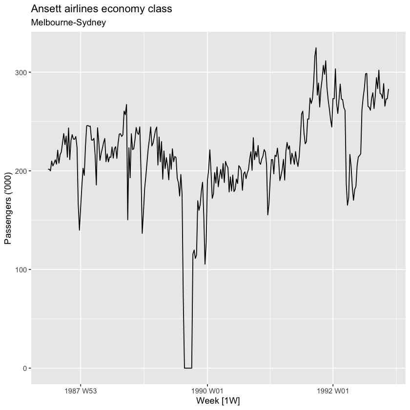
melsyd_economy <- tsibbledata::ansett %>%
  filter(Airports == 'MEL-SYD', Class == 'Economy') %>%
  mutate(Passengers = Passengers / 100)

autoplot(melsyd_economy, Passengers) +
  labs(
    title    = "Ansett airlines economy class",
    subtitle = 'Melbourne-Sydney',
    y        = "Passengers ('000)"
  )

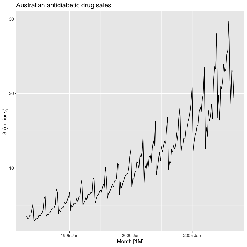
autoplot(a10, Cost) +
  labs(
    y     = '$ (millions)',
    title = 'Australian antidiabetic drug sales'
  )

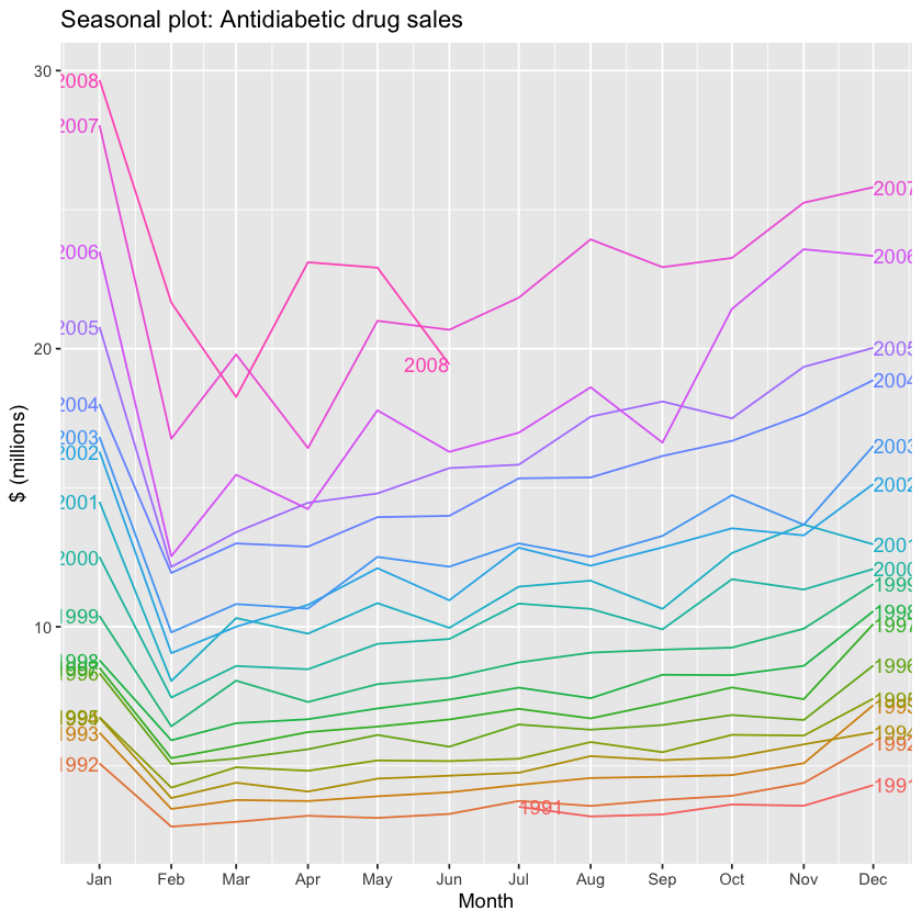
2.4 Seasonal plots

a10 %>%
  gg_season(Cost, labels = 'both') +
    labs(
      y     = '$ (millions)',
      title = 'Seasonal plot: Antidiabetic drug sales'
    )

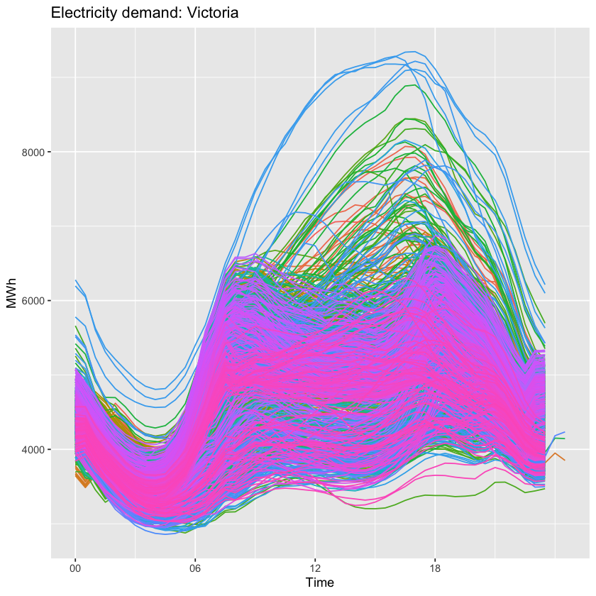
tsibbledata::vic_elec %>%
  gg_season(Demand, period = 'day') +
    theme(legend.position = 'none') +
    labs(
      y     = 'MWh',
      title = 'Electricity demand: Victoria'
    )

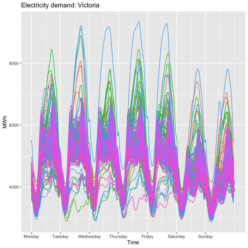
tsibbledata::vic_elec %>%
  gg_season(Demand, period = 'week') +
    theme(legend.position = 'none') +
    labs(
      y     = 'MWh',
      title = 'Electricity demand: Victoria'
    )

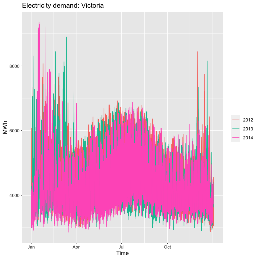
tsibbledata::vic_elec %>%
  gg_season(Demand, period = 'year') +
    labs(
      y     = 'MWh',
      title = 'Electricity demand: Victoria'
    )

2.5 Seasonal subseries plots

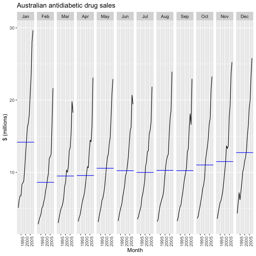
a10 %>%
  gg_subseries(Cost) +
    labs(
      y     = '$ (millions)',
      title = 'Australian antidiabetic drug sales'
    )

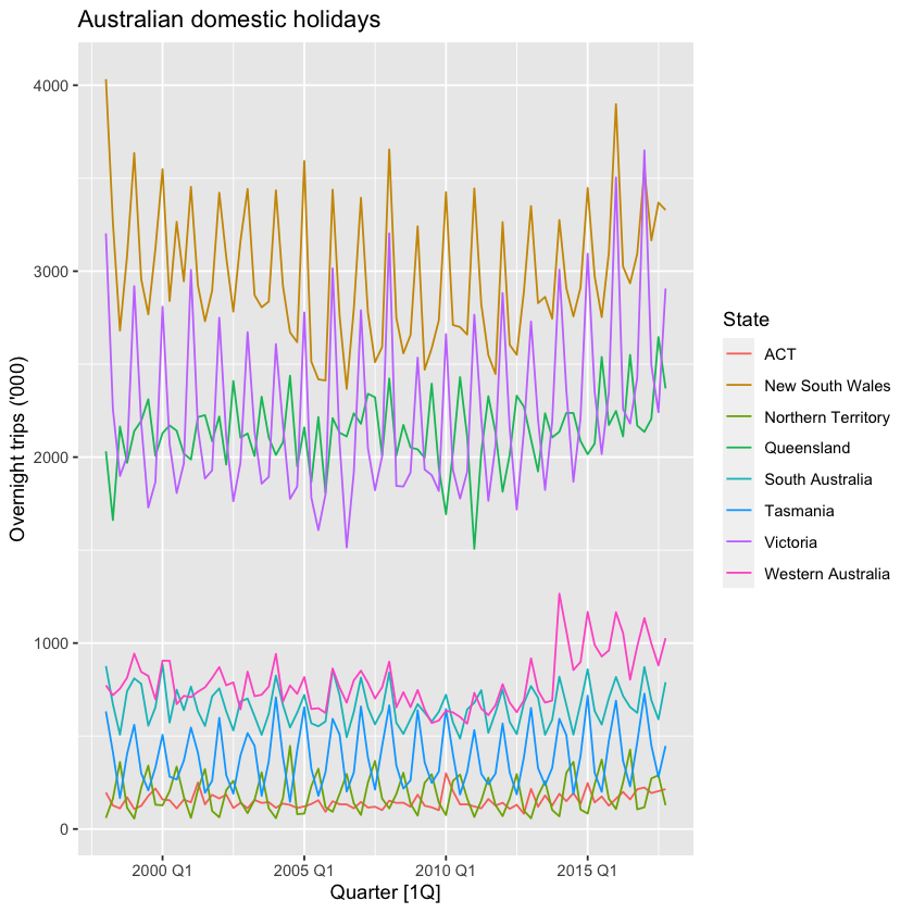
holidays <- tsibble::tourism %>%
  filter(Purpose == 'Holiday') %>%
  group_by(State) %>%
  summarize(Trips = sum(Trips))
head(holidays)

A tbl_ts: 6 × 3

State	Quarter	Trips
<chr>	<qtr>	<dbl>
ACT	1998 Q1	196.2186
ACT	1998 Q2	126.7706
ACT	1998 Q3	110.6796
ACT	1998 Q4	170.4722
ACT	1999 Q1	107.7792
ACT	1999 Q2	124.6442

autoplot(holidays, Trips) +
  labs(
    y     = "Overnight trips ('000)",
    title = 'Australian domestic holidays'
  )

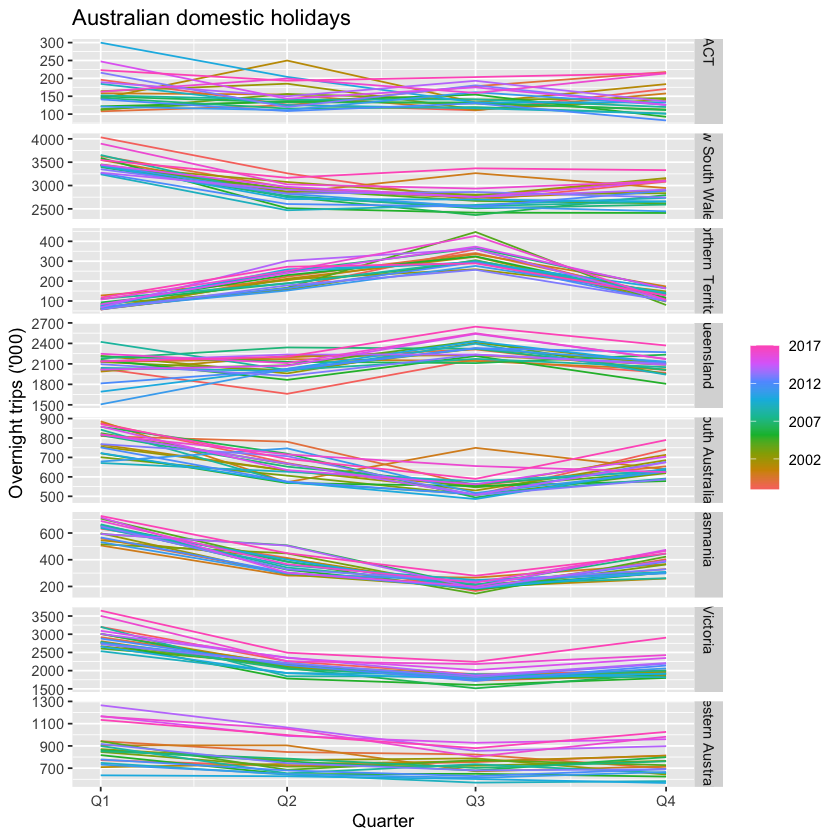
gg_season(holidays, Trips) +
  labs(
    y     = "Overnight trips ('000)",
    title = 'Australian domestic holidays'
  )

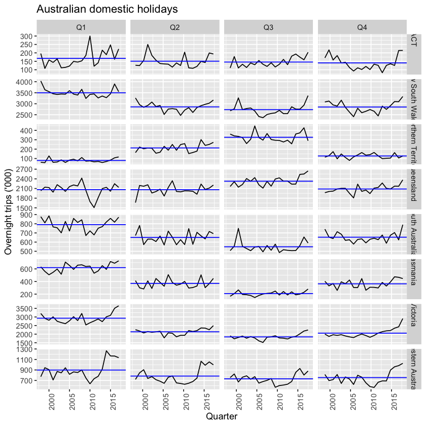
gg_subseries(holidays, Trips) +
  labs(
    y     = "Overnight trips ('000)",
    title = 'Australian domestic holidays'
  )

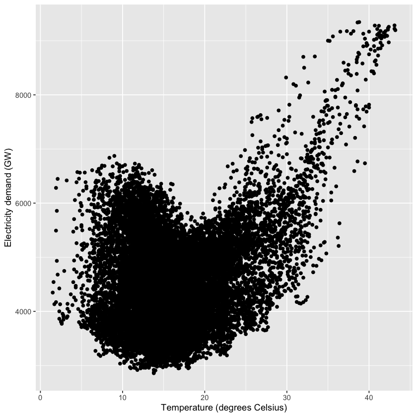
2.6 Scatterplots

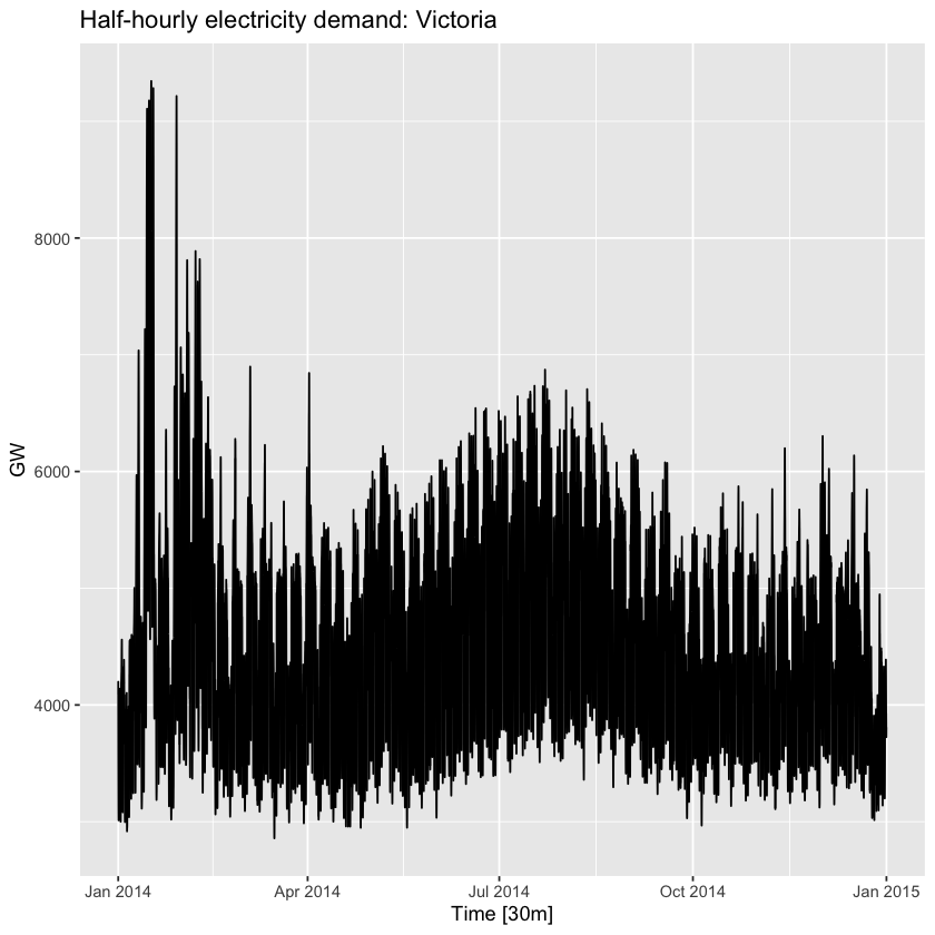
tsibbledata::vic_elec %>%
  filter(year(Time) == 2014) %>%
  autoplot(Demand) +
    labs(
      y     = 'GW',
      title = 'Half-hourly electricity demand: Victoria'
    )

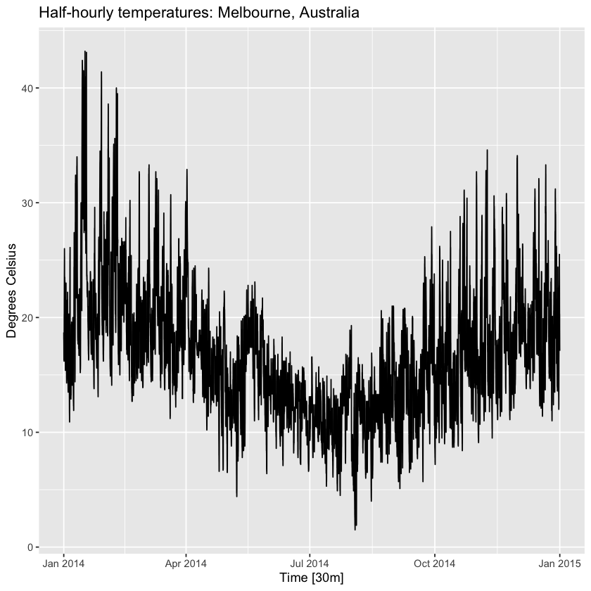
tsibbledata::vic_elec %>%
  filter(year(Time) == 2014) %>%
  autoplot(Temperature) +
    labs(
      y     = 'Degrees Celsius',
      title = 'Half-hourly temperatures: Melbourne, Australia'
    )

tsibbledata::vic_elec %>%
  filter(year(Time) == 2014) %>%
  ggplot(aes(x = Temperature, y = Demand)) +
    geom_point() +
    labs(
      x = 'Temperature (degrees Celsius)',
      y = 'Electricity demand (GW)'
    )

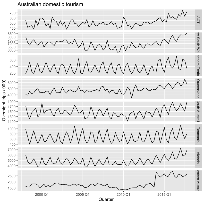
visitors <- tsibble::tourism %>%
  group_by(State) %>%
  summarize(Trips = sum(Trips))

visitors %>%
  ggplot(aes(x = Quarter, y = Trips)) +
    geom_line() +
    facet_grid(vars(State), scales = 'free_y') +
    labs(
      title = 'Australian domestic tourism',
      y     = "Overnight trips ('000)"
    )

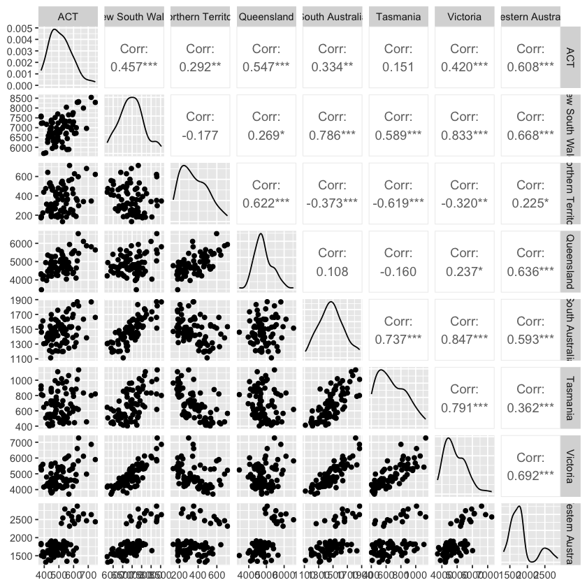
visitors %>%
  pivot_wider(values_from = Trips, names_from = State) %>%
  GGally::ggpairs(columns = 2:9)

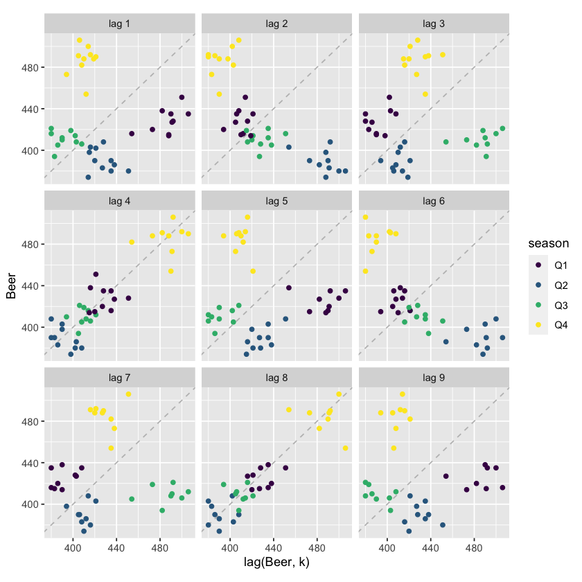
2.7 Lag plots

recent_production <- tsibbledata::aus_production %>%
  filter(year(Quarter) >= 2000)
recent_production %>%
  gg_lag(Beer, geom = 'point') +
    labs(
      x = 'lag(Beer, k)'
    )

2.8 Autocorrelation

recent_production %>%
  ACF(Beer, lag_max = 9)

A tbl_cf: 9 × 2

lag	acf
<cf_lag>	<dbl>
1Q	-0.052981076
2Q	-0.758175440
3Q	-0.026233757
4Q	0.802204530
5Q	-0.077471204
6Q	-0.657451271
7Q	0.001194922
8Q	0.707254078
9Q	-0.088756255

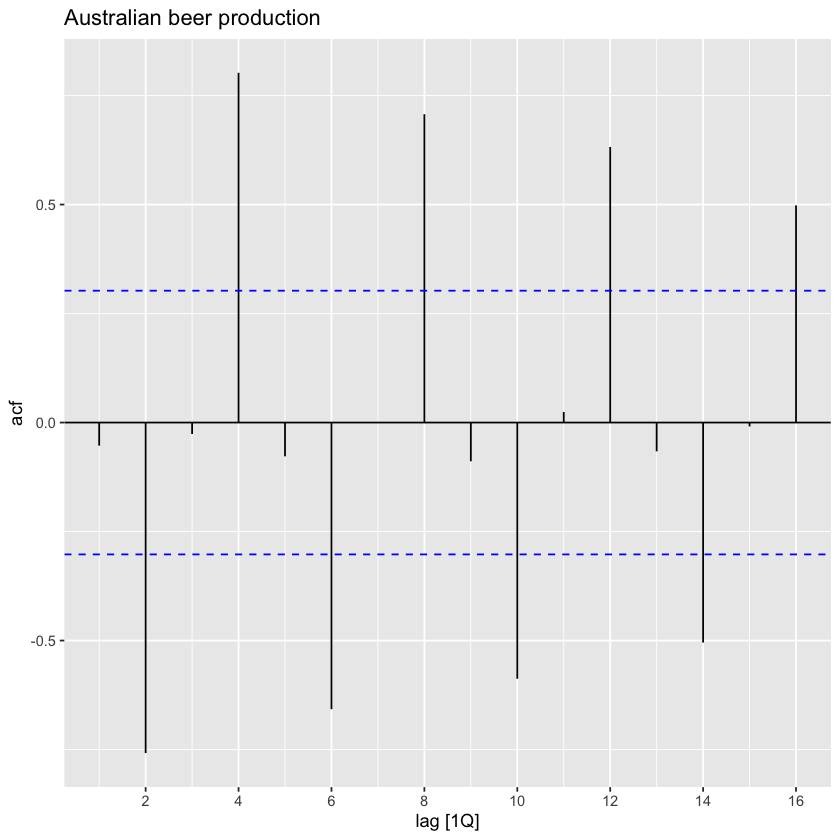
recent_production %>%
  ACF(Beer) %>%
  autoplot() +
    labs(
      title = 'Australian beer production'
    )

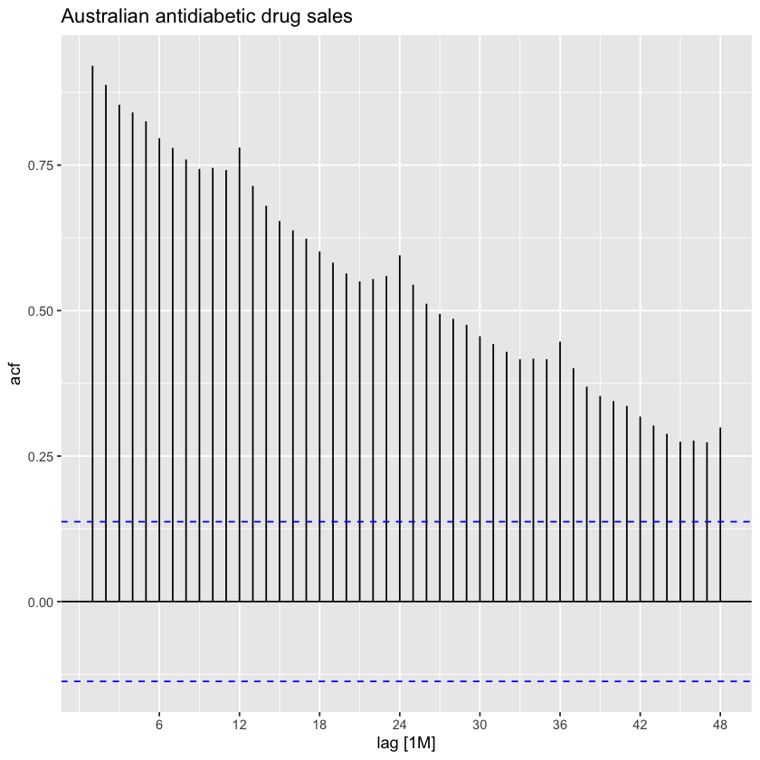
a10 %>%
  ACF(Cost, lag_max = 48) %>%
  autoplot() +
    labs(
      title = 'Australian antidiabetic drug sales'
    )

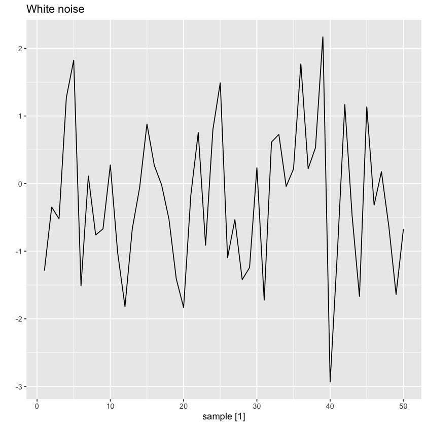
2.9 White noise

set.seed(30)

y <- tsibble(
  sample = 1:50,
  wn     = rnorm(50),
  index  = sample
)

y %>%
  autoplot(wn) +
    labs(
      title = 'White noise',
      y     = ''
    )

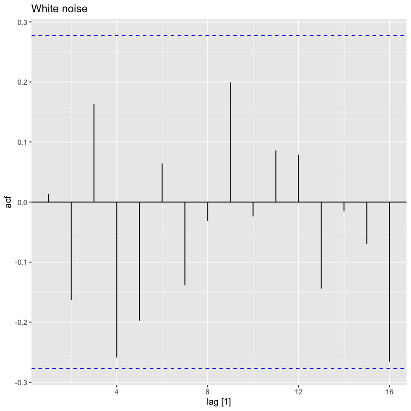
y %>%
  ACF(wn) %>%
  autoplot() +
    labs(
      title = 'White noise'
    )

3 - Time series decomposition

3.1 Transformations and adjustments

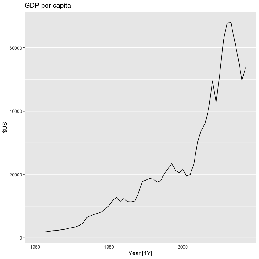
tsibbledata::global_economy %>%
  filter(Country == 'Australia') %>%
  autoplot(GDP/Population) +
    labs(
      title = 'GDP per capita',
      y     = '$US'
    )

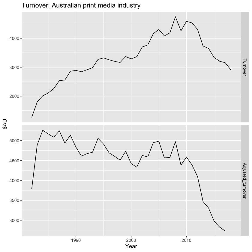
print_retail <- tsibbledata::aus_retail %>%
  filter(Industry == 'Newspaper and book retailing') %>%
  group_by(Industry) %>%
  index_by(Year = year(Month)) %>%
  summarize(Turnover = sum(Turnover))
  
aus_economy <- tsibbledata::global_economy %>%
  filter(Code == 'AUS')

print_retail %>%
  left_join(aus_economy, by = 'Year') %>%
  mutate(Adjusted_turnover = Turnover / CPI * 100) %>%
  pivot_longer(c(Turnover, Adjusted_turnover), values_to = 'Turnover') %>%
  mutate(name = factor(name, levels = c('Turnover', 'Adjusted_turnover'))) %>%
  ggplot(aes(x = Year, y = Turnover)) +
    geom_line() +
    facet_grid(name ~ ., scales = 'free_y') +
    labs(
      title = 'Turnover: Australian print media industry',
      y     = '$AU'
    )

Warning message:
“Removed 1 row containing missing values (`geom_line()`).”

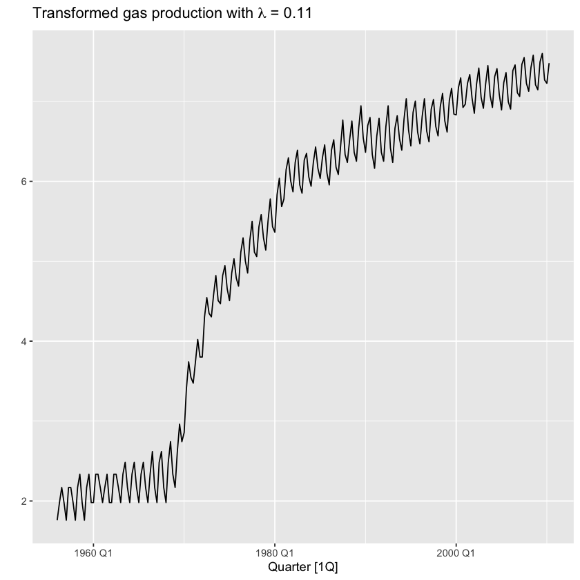
lambda <- tsibbledata::aus_production %>%
  features(Gas, features = guerrero) %>%
  pull(lambda_guerrero)

tsibbledata::aus_production %>%
  autoplot(box_cox(Gas, lambda)) +
  labs(
    y = '',
    title = latex2exp::TeX(paste0('Transformed gas production with $\\lambda$ = ', round(lambda, 2)))
  )

---

Bibliography

Hyndman, Rob J. & George Athanasopoulos. (2021). Forecasting: Principles and Practice. 3rd Ed. OTexts. Home.

---