Analysis of Speech Sounds#
Based on Chs. 6,7,8,9 of Johnson, Keith. (2012). Acoustic and Auditory Phonetics. 3rd Ed. Wiley-Blackwell.
Programming Environment#
Show code cell source
import numpy                    as np
np.set_printoptions(suppress=True) # suppress scientific notation
import numpy.random             as npr
import pandas                   as pd

import matplotlib               as mpl
import matplotlib.pyplot        as plt
plt.style.use('ggplot');

from   html.entities import codepoint2name
import string
import unicodedata

from   datetime import datetime as d
import locale                   as l
import platform                 as p
import sys                      as s

pad = 20
print(f"{'Executed'.upper():<{pad}}: {d.now()}")
print()
print(f"{'Platform'        :<{pad}}: "
      f"{p.mac_ver()[0]} | "
      f"{p.system()} | "
      f"{p.release()} | "
      f"{p.machine()}")
print(f"{''                :<{pad}}: {l.getpreferredencoding()}")
print()
print(f"{'Python'          :<{pad}}: {s.version}")
print(f"{''                :<{pad}}: {s.version_info}")
print(f"{''                :<{pad}}: {p.python_implementation()}")
print()
print(f"{'Matplotlib'      :<{pad}}: {mpl.__version__}")
print(f"{'NumPy'           :<{pad}}: { np.__version__}")
print(f"{'Pandas'          :<{pad}}: { pd.__version__}")
EXECUTED            : 2024-05-21 15:45:15.570576

Platform            : 14.4.1 | Darwin | 23.4.0 | arm64
                    : UTF-8

Python              : 3.11.9 | packaged by conda-forge | (main, Apr 19 2024, 18:34:54) [Clang 16.0.6 ]
                    : sys.version_info(major=3, minor=11, micro=9, releaselevel='final', serial=0)
                    : CPython

Matplotlib          : 3.8.4
NumPy               : 1.26.4
Pandas              : 2.2.2
Vowels#
Based on Ch 6 of Keith Johnson’s Acoustic and Auditory Phonetics.
Tube Models of Vowel Production#
Tube models of vowel production
vocal tract as cylinder
Source-Filter Theory
the prediction of resonant frequencies of the vocal tract (formants), assuming that the cross-sectional area of the tube is uniform
the resonant frequencies as a function of tube length
lengthening of the tube
lip protrusion
larynx lowering
vocal tract as a set of tubes of varying width
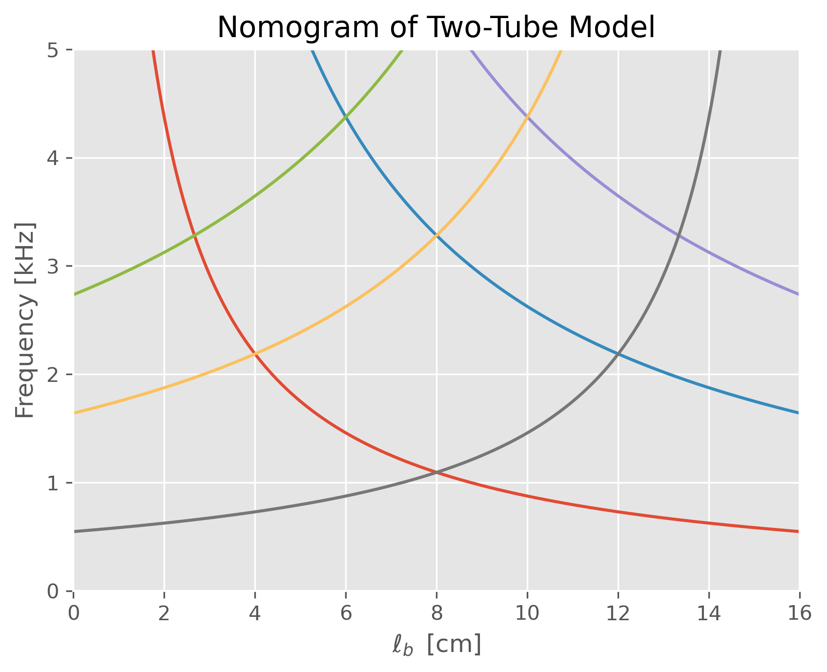
Two-Tube Model#
[Stevens 1989]
The vocal tract is modeled as the set of two uniform tubes.

back tube b, open at one end and closed at one end
    lb length
    Ab cross-sectional area
    closed at the glottis
    open at the junction with the front tube

front tube f, open at one end and closed at one end
    lf length
    Af cross-sectional area
    closed at the junction with the back tube
    open at the lips
\(A_b\lt\lt A_f\)
\( \begin{aligned} \text{resonances of the back cavity}\,\,\, F_{bn} &=\frac{(2n-1)c}{4l_b} \\ \text{resonances of the front cavity}\,\,\, F_{fn} &=\frac{(2n-1)c}{4l_f} \end{aligned} \)
Show code cell source
fig = plt.figure(dpi=300);
ax  = plt.subplot();
#ax.set_aspect(1);

def Fb (n,lb,L=16,c=35e3):
  return (2*n-1)*c/(4*lb)
def Ff (n,lf,L=16,c=35e3):
  return (2*n-1)*c/(4*(L-lf))

x=np.linspace(1e-3,16-1e-3,1001)
fb1=Fb(1,x)
fb2=Fb(2,x)
fb3=Fb(3,x)
ff1=Ff(1,x)
ff2=Ff(2,x)
ff3=Ff(3,x)

ax.plot(x,fb1);
ax.plot(x,fb2);
ax.plot(x,fb3);
ax.plot(x,ff1);
ax.plot(x,ff2);
ax.plot(x,ff3);

ax.set_yticks(ticks =[0,1e3,2e3,3e3,4e3,5e3],
              labels=[0,1,2,3,4,5]);
ax.set_xlim(0,16);
ax.set_ylim(0,5e3);
ax.set_xlabel('$\ell_b\,\,\,\mathrm{[cm]}$');
ax.set_ylabel('Frequency [kHz]');
ax.set_title('Nomogram of Two-Tube Model');
L=8
print(Ff(1,L))
print(Ff(2,L))
print(Ff(3,L))
1093.75
3281.25
5468.75
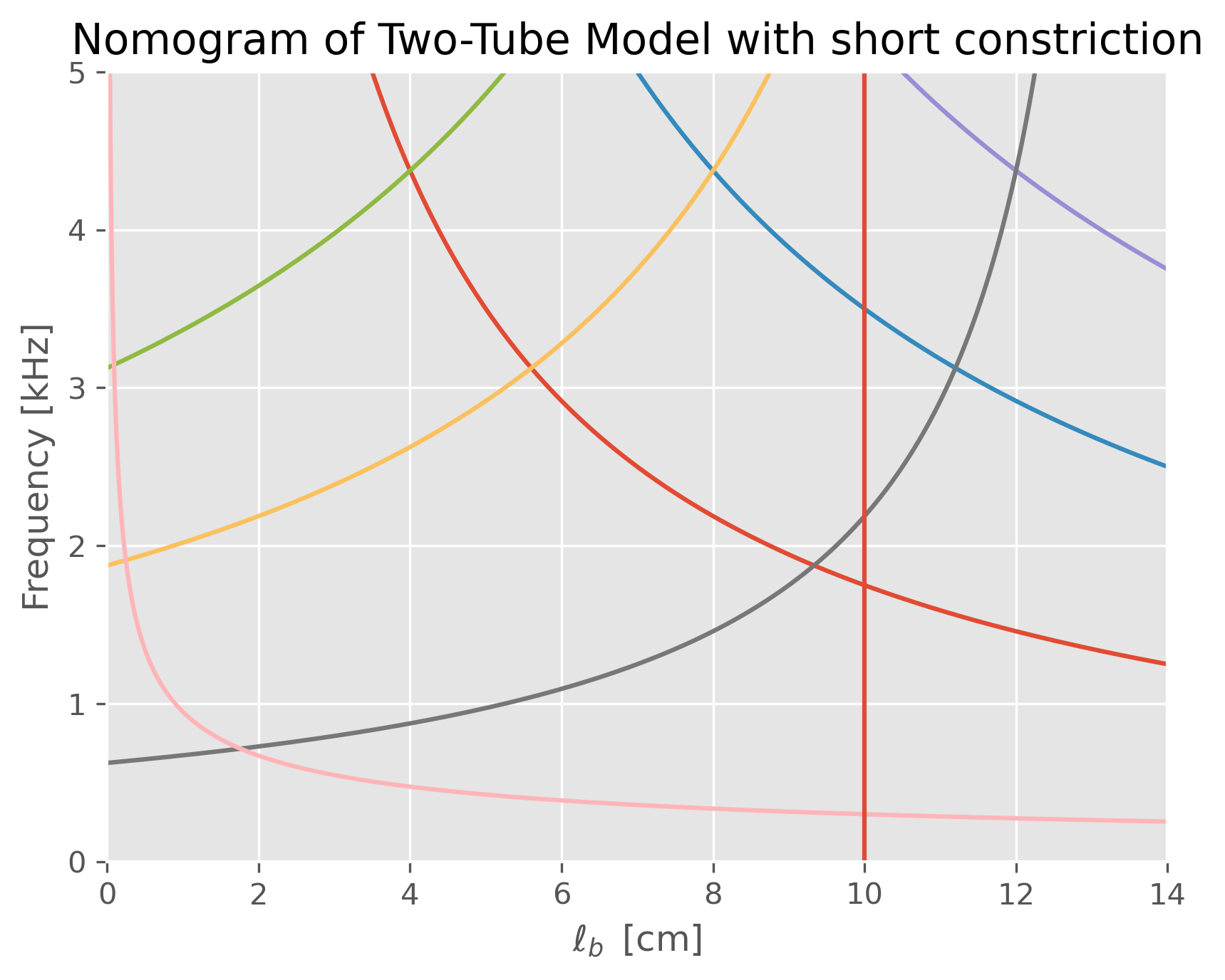
Two-Tube Model with short constriction#
The vocal tract is modeled as the set of three uniform tubes, where the third represents a short constriction.

back tube b, closed at both ends
    lb length
    Ab cross-sectional area
    closed at the glottis
    closed at the constriction

front tube f, open at one end and closed at one end
    lf length
    Af cross-sectional area
    closed at the constriction
    open at the lips

short constriction
    lc length
    Ac cross-sectional area
\( \begin{aligned} F_{n} &=\frac{(2n-1)c}{4L} &&\text{uniform tube closed at one end and open at one end} \\ F_{n} &=\frac{nc}{2L} &&\text{uniform tube closed at both ends} \\ f &=\frac{c}{2\pi}\sqrt{\frac{A_c}{A_bl_bl_c}} &&\text{Helmholtz resonance} \end{aligned} \)
\( \begin{aligned} f &=\frac{c}{2\pi}\sqrt{\frac{A_c}{A_bl_bl_c}} \\ \frac{A_c}{A_b} &=l_bl_c\left(\frac{2\pi f}{c}\right)^2 \\ &=(10)(2)\left(\frac{2\pi(300)}{35000}\right)^2 \end{aligned} \)
20*(2*np.pi*300/35e3)**2
0.058009103418647644
Show code cell source
fig = plt.figure(dpi=300);
ax  = plt.subplot();
#ax.set_aspect(1);

def Fb (n,lb,c=35e3):
  return n*c/(2*lb)

def Ff (n,lb,lc=2,L=16,c=35e3):
  return (2*n-1)*c/(4*(L-lc-lb))

def Fh (lb,lc=2,c=35e3):
  return (c/2/np.pi)*np.sqrt(0.58e-1/lb/lc)

e=1e-3
x=np.linspace(e,14-e,1001)
fb1=Fb(1,x)
fb2=Fb(2,x)
fb3=Fb(3,x)
ff1=Ff(1,x)
ff2=Ff(2,x)
ff3=Ff(3,x)
fh =Fh(  x)

ax.plot(x,fb1);
ax.plot(x,fb2);
ax.plot(x,fb3);
ax.plot(x,ff1);
ax.plot(x,ff2);
ax.plot(x,ff3);
ax.plot(x, fh);

ax.axvline(10);

ax.set_yticks(ticks =[0,1e3,2e3,3e3,4e3,5e3],
              labels=[0,1,2,3,4,5]);
ax.set_xlim(0,14);
ax.set_ylim(0,5e3);
ax.set_xlabel('$\ell_b\,\,\,\mathrm{[cm]}$');
ax.set_ylabel('Frequency [kHz]');
ax.set_title('Nomogram of Two-Tube Model with short constriction');
L=10
print(Fh(L))
print(Fb(1,L))
print(Ff(1,L))
299.97645944698934
1750.0
2187.5
Perturbation Theory#
air pressure vs velocity
Acoustic Vowel Space#
[i]
    low  F1   high/close
    high F2   front

[a]
    high F1   low/open
    low  F2   back

[u]
    low  F1   high/close
    low  F2   back

F3
    rhotic
    acoustic cue for the front rounded vowels
Fricatives#
Stops and Affricates#
Nasals and Laterals#
Resources#
Terms#
Bibliography#
Johnson, Keith. (2012). Acoustic and Auditory Phonetics. 3rd Ed. Wiley-Blackwell.