Conic Sections#
Revised
19 Feb 2023
Imports & Environment#
Show code cell source
# %load imports.py
import numpy                    as np
import numpy.random             as npr
import pandas                   as pd

import matplotlib               as mpl
mpl.rcParams['lines.color'] = 'k'
mpl.rcParams['axes.prop_cycle'] = mpl.cycler('color',['k'])
from   matplotlib import cm
from   matplotlib.patches import Ellipse
import matplotlib.pyplot        as plt
plt.style.use('ggplot');
from   matplotlib.ticker import LinearLocator

import plotly
import plotly.express           as px
import plotly.graph_objects     as go

import sympy as sy
from   sympy.geometry import Point, Line
from   sympy import (diff,
                     dsolve,
                     Eq,
                     expand,
                     factor,
                     Function,
                     init_printing,
                     Integer,
                     Integral,
                     integrate,
                     latex,
                     limit,
                     Matrix,
                     Poly,
                     Rational,
                     solve,
                     Symbol,
                     symbols)

S =Symbol
ss=symbols
x,y,z,t,u,v=ss(names='x y z t u v')
init_printing(use_unicode=True)

import math
import numexpr

from   datetime import datetime as d
import locale                   as l
import platform                 as p
import sys                      as s

pad = 20
print(f"{'Executed'.upper():<{pad}}: {d.now()}")
print()
print(f"{'Platform'        :<{pad}}: "
      f"{p.mac_ver()[0]} | "
      f"{p.system()} | "
      f"{p.release()} | "
      f"{p.machine()}")
print(f"{''                :<{pad}}: {l.getpreferredencoding()}")
print()
print(f"{'Python'          :<{pad}}: {s.version}")
print(f"{''                :<{pad}}: {s.version_info}")
print(f"{''                :<{pad}}: {p.python_implementation()}")
print()
print(f"{'Matplotlib'      :<{pad}}: {mpl.__version__}")
print(f"{'Numexpr'         :<{pad}}: {numexpr.__version__}")
print(f"{'NumPy'           :<{pad}}: {np.__version__}")
print(f"{'Pandas'          :<{pad}}: {pd.__version__}")
print(f"{'Plotly'          :<{pad}}: {plotly.__version__}")
print(f"{'SymPy'           :<{pad}}: {sy.__version__}")
# print()
# from pprint import PrettyPrinter
# pp = PrettyPrinter(indent=2)
# pp.pprint([name for name in dir()
#            if name[0] != '_'
#            and name not in ['In', 'Out', 'exit', 'get_ipython', 'quit']])
---------------------------------------------------------------------------
ModuleNotFoundError                       Traceback (most recent call last)
Cell In[1], line 46
     43 init_printing(use_unicode=True)
     45 import math
---> 46 import numexpr
     48 from   datetime import datetime as d
     49 import locale                   as l

ModuleNotFoundError: No module named 'numexpr'
Auxiliary code#
x=np.linspace(-9,9,400)
y=np.linspace(-9,9,400)
x,y=np.meshgrid(x,y)

def axes ():
  plt.axhline(0,alpha=0.1)
  plt.axvline(0,alpha=0.1)
Linear Equation#
linear in \(n\) variables \(x_1,...,x_n\)
\(a_1x_1+a_2x_2+...+a_nx_n=b\)
linear in two variables \(x,y\)
Standard Form of a Line
\(Ax+By=C\)
Point-Slope Form
\(y-y_0=m(x-x_0)\) for point \((x_0,y_0)\) and slope \(m\)
Slope-Intercept Form
\(y=mx+b\)
\( \begin{aligned} Ax+By=C \implies By=-Ax+C \implies y=-\frac{A}{B}x+\frac{C}{B} \implies y=mx+b\,\,\,\text{where}\,\,\,m=-\frac{A}{B}\,\,\,\text{and}\,\,\,b=\frac{B}{C} \end{aligned} \)
General quadratic in a single variable#
General form of a quadratic equation in a single variable \(x\)
\(Ax^2+Bx+C=0\) where \(A\ne0\)
General quadratic in two variables#
General form of a quadratic equation in two variables \(x,y\)
with cross terms
\(Ax^2+Bxy+Cy^2+Dx+Ey+F=0\) where \(A\ne0\lor B\ne0\lor C\ne0\)
without cross terms
\(Ax^2+By^2+Cx+Dy+E=0\) where \(A\ne0\lor B\ne0\)
Conics#
Parabola
\( (y-k)=a(x-h)^2 \)
Ellipse
\( \begin{aligned} \left(\frac{x-h}{a}\right)^2+\left(\frac{y-k}{b}\right)^2=1 \end{aligned} \)
Hyperbola
\( \begin{aligned} \left(\frac{x-h}{a}\right)^2-\left(\frac{y-k}{b}\right)^2&=1\\ \left(\frac{y-k}{b}\right)^2-\left(\frac{x-h}{a}\right)^2&=1\\ \end{aligned} \)
Parabola#
Standard Form of a Parabola#
Start with the general quadratic in two variables \(x,y\) ignoring cross terms
\( Ax^2+By^2+Cx+Dy+E=0 \) where \(A=0\lor B=0\)
\(Ax^2+Cx+Dy+E=0\)
or
\(By^2+Cx+Dy+E=0\)
Complete the square
\( \begin{aligned} Ax^2+Cx+Dy+E&=0\\ \implies\\ -Dy-E&=Ax^2+Cx\\ \implies\\ -Dy-E&=A\left(x^2+\frac{C}{A}x\right)\\ \implies\\ -Dy-E&=A\left(\left(x+\frac{C}{2A}\right)^2-\left(\frac{C}{2A}\right)^2\right)\\ \implies\\ -Dy-E&=A\left(x+\frac{C}{2A}\right)^2-\frac{C^2}{4A}\\ \implies\\ -Dy-E+\frac{C^2}{4A}&=A\left(x+\frac{C}{2A}\right)^2\\ \implies\\ y+\frac{E}{D}-\frac{C^2}{4AD}&=-\frac{A}{D}\left(x+\frac{C}{2A}\right)^2\\ \implies\\ y-\left(\frac{C^2}{4AD}-\frac{E}{D}\right)&=-\frac{A}{D}\left(x-\left(-\frac{C}{2A}\right)\right)^2\\ \implies\\ y-k&=a\left(x-h\right)^2\\ \end{aligned} \)
where
\(k=\left(\frac{C^2}{4AD}-\frac{E}{D}\right)\)
\(a=-\frac{A}{D}\)
\(h=\left(-\frac{C}{2A}\right)\)
Standard Form of a Parabola
\((y-k)=a(x-h)^2\) is \(y=x^2\) shifted right \(h\) units; shifted up \(k\) units; and stretched vertically by a factor of \(a\); with vertex \((h,k)\)
as a function
\(y=a(x-h)^2+k\)
find the vertex via differentiation to see where the graph has a horizontal tangent line
\( \begin{aligned} y &=a(x-h)^2+k\\ &=ax^2-2ahx+ah^2+k\implies\\ y'&=2ax-2ah\\ 0&=2ax-2ah\implies\\ x&=h\implies y=k\\ \end{aligned} \)
complete the square in the squared variable to find the vertex
plug the vertex into the equation \(y=ax^2+bx+c\) to find the y-intercept
factor the equation to find any roots
a parabola has an axis of symmetry through its vertex; therefore, any point on one side of the parabola is informative of a point on the other side
when the squared variable is y, then the graph is a shifted and stretched version of \(x=y^2\)
in this case, the parabola always has an x-intercept and the roots of the parabola are y-intercepts
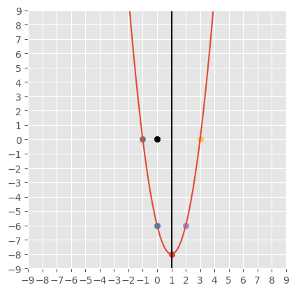
[EXAMPLE]
\( \begin{aligned} 2x^2-4x-y=6 &\implies y+6=2x^2-4x\\ &\implies y+6=2(x^2-2x)\\ &\implies y+6=2((x-1)^2-1)\\ &\implies y+6=2(x-1)^2-2\\ &\implies y+8=2(x-1)^2\\ \end{aligned} \)
vertex
\((h,k)=(1,-8)\)
\( \begin{aligned} 2x^2-4x-y=6 &\implies y=2x^2-4x-6\\ x=0&\implies y=-6\\ \end{aligned} \)
y-intercept
\((0,y)=(0,-6)\)
\( \begin{aligned} 2x^2-4x-y=6 &\implies y=2x^2-4x-6\\ &\implies y=2(x^2-2x-3)\\ &\implies y=2(x-3)(x+1)\\ \end{aligned} \)
roots (x-intercepts)
\(x-3=0\implies x=3\)
\(x+1=0\implies x=-1\)
by symmetry
\((2h,y)=(2,-6)\)
Show code cell source
s=9
x=np.linspace(-s,s,1001);
y=2*x**2-4*x-6

plt.axes().set_aspect(1);
plt.xlim((-s,s));
plt.xticks(np.arange(-s,s+1,1));
plt.ylim((-s,s));
plt.yticks(np.arange(-s,s+1,1));

plt.plot(x,y);
plt.scatter(0,0,color='black');
plt.axvline(x=1,color='black');
plt.scatter( 1,-8);
plt.scatter( 0,-6);
plt.scatter( 2,-6);
plt.scatter(-1, 0);
plt.scatter( 3, 0);
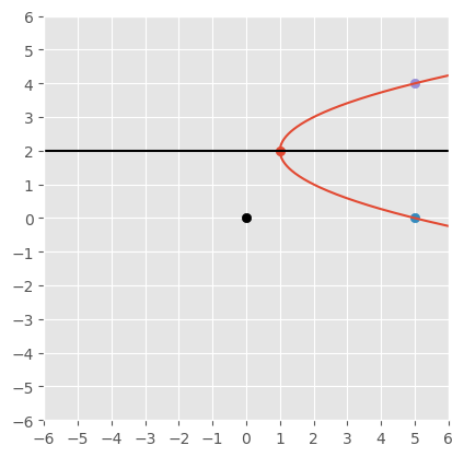
[EXAMPLE]
\( \begin{aligned} x+4y=y^2+5 &\implies x=y^2-4y+5\\ &\implies x=(y-2)^2+1\\ &\implies x-1=(y-2)^2\\ \end{aligned} \)
vertex
\((h,k)=(1,2)\)
\( \begin{aligned} x+4y=y^2+5 &\implies x=y^2-4y+5\\ y=0&\implies x=5\\ \end{aligned} \)
x-intercept
\((x,0)=(5,0)\)
roots (y-intercepts)
\( \begin{aligned} y=\frac{-b\pm\sqrt{b^2-4ac}}{a^2} &\implies y=\frac{-(-4)\pm\sqrt{(-4)^2-4(1)(5)}}{(1)^2}\\ &\implies y=4\pm\sqrt{16-20}\\ &\implies y=4\pm2\sqrt{-1}\\ &\implies y=4\pm2i\\ \end{aligned} \)
by symmetry
\((x,2k)=(5,4)\)
Show code cell source
s=6
y=np.linspace(-s,s,1001);
x=y**2-4*y+5

plt.axes().set_aspect(1);
plt.xlim((-s,s));
plt.xticks(np.arange(-s,s+1,1));
plt.ylim((-s,s));
plt.yticks(np.arange(-s,s+1,1));

plt.plot(x,y);
plt.scatter(0,0,color='black');
plt.axhline(y=2,color='black');
plt.scatter(1,2);
plt.scatter(5,0);
plt.scatter(5,4);
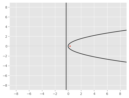
\( y^2=4ax \) where \(a\gt0\)
focus \((a,0)\)
directrix \(x=-a\)
Example in standard position#
Show code cell source
x=np.linspace(-9,9,400)
y=np.linspace(-9,9,400)
x,y=np.meshgrid(x,y)

def axes ():
  plt.axhline(0,alpha=0.1)
  plt.axvline(0,alpha=0.1)

a=0.3
axes()
plt.contour(x,y,y**2-4*a*x,[0],colors='k');
# focus
plt.plot(a,0,'.');
# directrix
plt.axvline(-a);
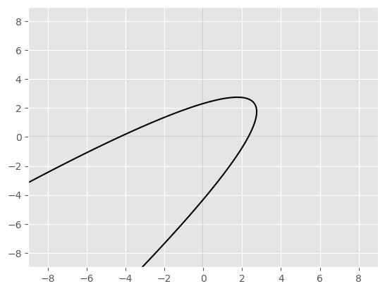
Non Standard Form of a Parabola#
Start with the general quadratic in two variables \(x,y\)
\( Ax^2+Bxy+Cx^2+Dx+Ey+F=0 \) where \(B^2-4AC=0\)
Example in non standard position#
Show code cell source
a=  1
b= -2
c=  1
d=  2
e=  2
f=-10
assert b**2 - 4*a*c == 0

general=a*x**2 + b*x*y + c*y**2 + d*x + e*y + f

axes()
plt.contour(x,y,general,[0],colors='k');
Ellipse#
\( \boxed{ \begin{aligned} A=\pi ab \end{aligned} } \)
Standard Form of an Ellipse#
Start with the general quadratic in two variables \(x,y\) ignoring cross terms
\( Ax^2+By^2+Cx+Dy+E=0 \) where \(A\ne0\land B\ne0\) and \(A\) and \(B\) have the same sign
Complete the square in each variable separately to transform the general equation into the standard form of an ellipse.
\( \begin{aligned} Ax^2+By^2+Cx+Dy+E&=0\\ \implies\\ (Ax^2+Cx)+(By^2+Dy)&=-E\\ \implies\\ A\left(x^2+\frac{C}{A}x\right)+B\left(y^2+\frac{D}{B}y\right)&=-E\\ \implies\\ A\left(x^2+\frac{C}{A}x+\left(\frac{C}{2A}\right)^2\right)+B\left(y^2+\frac{D}{B}y+\left(\frac{D}{2B}\right)^2\right)&=-E+A\left(\frac{C}{2A}\right)^2+B\left(\frac{D}{2B}\right)^2\\ \implies\\ A\left(x+\frac{C}{2A}\right)^2+B\left(y+\frac{B}{2D}\right)^2&=\frac{C^2}{4A}+\frac{D^2}{4B}-E\\ \implies\\ A\left(x+\frac{C}{2A}\right)^2+B\left(y+\frac{B}{2D}\right)^2&=\frac{BC^2+AD^2-4ABE}{4AB}\\ \implies\\ \frac{4AB}{BC^2+AD^2-4ABE}\left(A\left(x+\frac{C}{2A}\right)^2+B\left(y+\frac{B}{2D}\right)^2\right)&=1\\ \implies\\ \frac{4A^2B}{BC^2+AD^2-4ABE}\left(x+\frac{C}{2A}\right)^2+\frac{4AB^2}{BC^2+AD^2-4ABE}\left(y+\frac{B}{2D}\right)^2&=1\\ \implies\\ ...\\ \end{aligned} \)
Standard Form of an Ellipse
\( \begin{aligned} \left(\frac{x-h}{a}\right)^2+\left(\frac{y-k}{b}\right)^2=1 \end{aligned} \)
\((h,k)\) center
\(a\) horizontal stretch factor
\(b\) vertical stretch factor
an ellipse centered at the origin
\( \begin{aligned} \frac{x^2}{a^2}+\frac{y^2}{b^2}=1 \end{aligned} \)
given the center of an ellipse
plug the x-coordinate of the center of the ellipse into the equation of the ellipse to find the y-coordinates of two points on the ellipse
plut the y-coordinate of the center of the ellipse into the equation of the ellipse to find the x-coordinates of two points on the ellipse
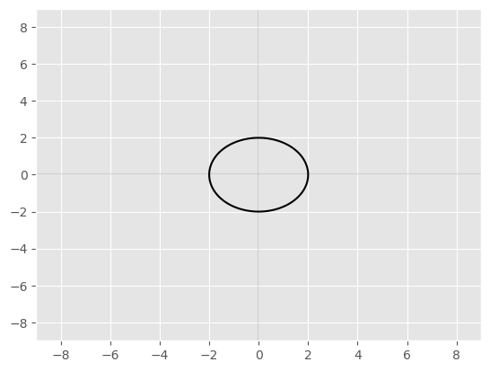
if \(a=b=r\), then the graph is a circle with radius \(r\)
\( \begin{aligned} \frac{x^2}{r^2}+\frac{y^2}{r^2}=1 \implies x^2+y^2=r^2 \end{aligned} \)
Unit Circle (radius \(r=1\))
\(x^2+y^2=1\)
center \((0,0)\)
[CASE]
Point (or Circle of radius \(r=0\))
[EXAMPLE]
\( \begin{aligned} (x-3)^2+(y+2)^2=0 &\implies (x-3)^2=0 \land (y+2)^2=0\\ &\implies x-3=0 \land y+2=0\\ &\implies x=3 \land y=-2\\ \end{aligned} \)
the only way for two square values to sum to zero is for each square itself to be equal to zero
[CASE]
DNE (or Circle with negative radius \(r\))
[EXAMPLE]
\( \begin{aligned} (x+4)^2+(y-1)^2=-2 \end{aligned} \)
two square values cannot sum to a negative number
[EXAMPLE]
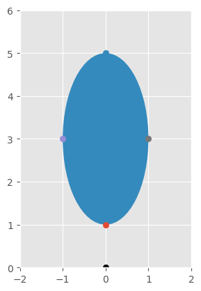
\( \begin{aligned} 4x^2+y^2=6y-5 &\implies4x^2+y^2-6y=-5\\ &\implies4(x^2)+(y^2-6y)=-5\\ &\implies4(x^2)+(y^2-6y+9)=-5+9\\ &\implies4(x^2)+(y-3)^2=4\\ &\implies x^2+\left(\frac{y-3}{2}\right)^2=1\\ \end{aligned} \)
center \((0,3)\)
\(a=1\)
\(b=2\)
\( \begin{aligned} x=0 &\implies y^2-6y+5=0\\ &\implies(y-5)(y-1)=0\\ &\implies y-5=0\land y-1=0\\ &\implies y=5\land y=1\\ \end{aligned} \)
\( \begin{aligned} y=3 &\implies 4x^2+(3)^2-6(3)=-5\\ &\implies x^2=1\\ &\implies x=\pm1\\ \end{aligned} \)
Show code cell source
h,k,a,b=0,3,1,2

fig,ax=plt.subplots(subplot_kw={'aspect':'equal'});
ax.add_artist(
  Ellipse(xy    =(h,k),
          width =2*a,
          height=2*b)
);
plt.scatter(0,0,color='black');
ax.set_xlim(h-a-1,h+a+1);
ax.set_ylim(k-b-1,k+b+1);

plt.scatter( 0,1);
plt.scatter( 0,5);
plt.scatter(-1,3);
plt.scatter( 1,3);
[EXAMPLE]
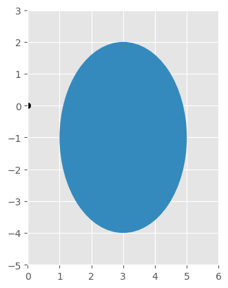
\( \begin{aligned} 9x^2+4y^2-54x+8y+49=0 &\implies (9x^2-54x)+(4y^2+8y)=-49\\ &\implies 9(x^2-6x)+4(y^2+2y)=-49\\ &\implies 9(x^2-6x+9)+4(y^2+2y+1)=-49+81+4\\ &\implies 9(x-3)^2+4(y+1)^2=36\\ &\implies \left(\frac{x-3}{2}\right)^2+\left(\frac{y+1}{3}\right)^2=1\\ \end{aligned} \)
\((3,-1)\) center
\(a=2,b=3\)
Show code cell source
h,k,a,b=3,-1,2,3

fig,ax=plt.subplots(subplot_kw={'aspect':'equal'});
ax.add_artist(
  Ellipse(xy    =(h,k),
          width =2*a,
          height=2*b)
);
plt.scatter(0,0,color='black');
ax.set_xlim(h-a-1,h+a+1);
ax.set_ylim(k-b-1,k+b+1);

# plt.scatter();
# plt.scatter();
# plt.scatter();
# plt.scatter();
Show code cell source
r=2

axes()
plt.contour(x,y,x**2/r**2 + y**2/r**2,[1],colors='k');
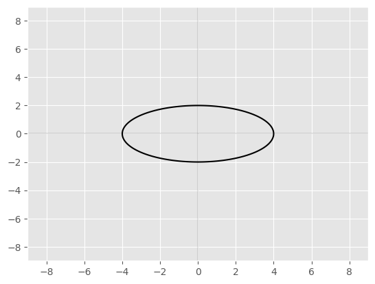
Show code cell source
a=4
b=2

axes()
plt.contour(x,y,x**2/a**2 + y**2/b**2,[1],colors='k');
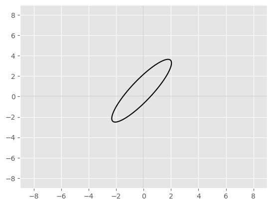
Nonstandard ellipse#
Start with the general quadratic in two variables \(x,y\)
\( Ax^2+Bxy+Cx^2+Dx+Ey+F=0 \) where \(B^2-4AC\lt0\)
Show code cell source
a=  4
b= -5
c=  2
d=  4
e= -3
f= -3
assert b**2 - 4*a*c < 0

general=a*x**2 + b*x*y + c*y**2 + d*x + e*y + f

axes()
plt.contour(x,y,general,[0],colors='k');
Hyperbola#
Start with the general quadratic in two variables \(x,y\) ignoring cross terms
\( Ax^2+By^2+Cx+Dy+E=0 \) where \(A\ne0\land B\ne0\) and \(A\) and \(B\) have opposite sign
Standard Forms of a Hyperbola
\( \begin{aligned} \left(\frac{x-h}{a}\right)^2-\left(\frac{y-k}{b}\right)^2&=1\\ \left(\frac{y-k}{b}\right)^2-\left(\frac{x-h}{a}\right)^2&=1\\ \end{aligned} \)
shifted to the right \(h\) units
shifted up \(k\) units
\(a\) horizontal scale factor
\(b\) vertical scale factor
\( \begin{aligned} x^2-y^2&=1\\ y^2-x^2&=1\\ \end{aligned} \)
Hyperbolas are not single, connected curves; but two symmetric branches. The point halfway beween them is \((h,k)\).
The graph of the hyperbola will approach the asymptotes as the graph goes to infinity.
Finding the equations of the asymptotes
standard form
set the left hand side equal to zero
simplify the equation via factoring or square roots
equations of two lines
Find the center \((h,k)\)
Plugin the x and y coordinates of the center into the equation, separately, and solve for the other coordinate
One of these coordinates will yield a pair of points; the other will not have solutions
These points determine whether the hyperbola opens horizontally or vertically
First, graph the asymptotes
[SPECIAL CASE]
The graph is just a pair of crossed lines
[EXAMPLE]
\( \begin{aligned} x^2-y^2-6x+8y-7&=0\\ \implies\\ (x^2-6x)-(y^2-8y)&=7\\ \implies\\ (x-3)^2-9-(y-4)^2+16&=7\\ \implies\\ (x-3)^2-(y-4)^2&=0\\ \implies\\ (x-3)^2&=(y-4)^2\\ \implies\\ \sqrt{(x-3)^2}&=\sqrt{(y-4)^2}\\ \implies\\ x-3&=\pm(y-4)\\ \implies\\ x-3&=y-4\\ x-3&=-(y-4)\\ \implies\\ y&=x+1\\ y&=-x+7\\ \end{aligned} \)
eccentricity \(e\)
\( \begin{aligned} e=\sqrt{1+\frac{b^2}{a^2}}\gt1 \end{aligned} \)
foci
directrices
asymptotes
\( \begin{aligned} y=\pm\frac{b}{a}x \end{aligned} \)
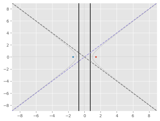
\( x^2-y^2=1 \)
Show code cell source
a = b = 1

# eccentricity
e = np.sqrt(1 + b**2/a**2)

# foci
plt.plot(a*e,0,'.',-a*e,0,'.');

# directrices
plt.axvline( a/e);
plt.axvline(-a/e);

# asymptotes
plt.plot(x[0,:], b/a*x[0,:],'--');
plt.plot(x[0,:],-b/a*x[0,:],'--');

eq = x**2/a**2 - y**2/b**2
axes()
plt.contour(x,y,eq,[1],colors='k',alpha=0.1);
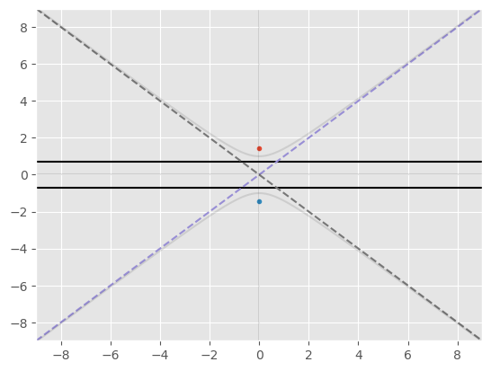
\( y^2-x^2=1 \)
Show code cell source
a = b = 1

# eccentricity
e = np.sqrt(1 + b**2/a**2)

# foci
plt.plot(0,a*e,'.',0,-a*e,'.');

# directrices
plt.axhline( a/e);
plt.axhline(-a/e);

# asymptotes
plt.plot(x[0,:], b/a*x[0,:],'--');
plt.plot(x[0,:],-b/a*x[0,:],'--');

eq = y**2/b**2 - x**2/a**2
axes()
plt.contour(x,y,eq,[1],colors='k',alpha=0.1);
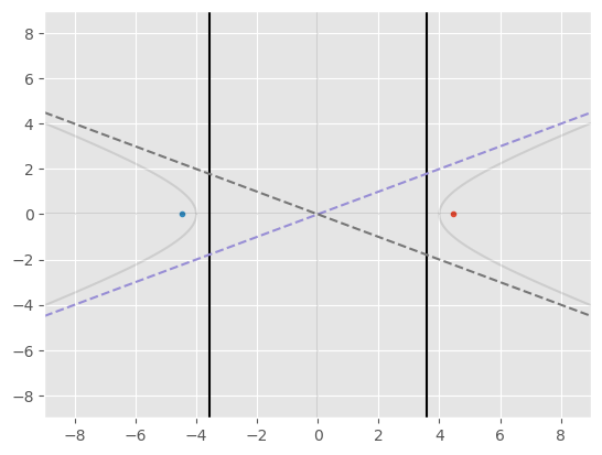
[EXAMPLE]
Determine the center
\( \begin{aligned} x^2-4y^2&=16\\ \implies\\ \frac{x^2}{16}-\frac{4y^2}{16}&=1\\ \implies\\ \left(\frac{x}{4}\right)^2-\left(\frac{y}{2}\right)^2&=1\\ \implies\\ (h,k)&=(0,0)\\ a,b&=4,2\\ \end{aligned} \)
Determine the intercepts
\( \begin{aligned} y=0 \implies x^2=16 \implies x=\pm\sqrt{16} \implies x=\pm4 \end{aligned} \)
\( \begin{aligned} x=0 \implies -4y^2=16 \implies y^2=-4 \implies y=\pm2\sqrt{-1} \implies \text{no real solutions} \end{aligned} \)
Determine the equations of the asymptotes
\( \begin{aligned} x^2-4y^2&=0\\ \implies\\ (x+2y)(x-2y)&=0\\ \implies\\ x+2y&=0\\ x-2y&=0\\ \implies\\ y&=-\frac{1}{2}x\\ y&=\frac{1}{2}x\\ \end{aligned} \)
Show code cell source
a,b,h,k=4,2,0,0

# eccentricity
e = np.sqrt(1 + b**2/a**2)

# foci
plt.plot(a*e,0,'.',-a*e,0,'.');

# directrices
plt.axvline( a/e);
plt.axvline(-a/e);

# asymptotes
plt.plot(x[0,:], b/a*x[0,:],'--');
plt.plot(x[0,:],-b/a*x[0,:],'--');

eq = x**2/a**2 - y**2/b**2
axes()
plt.contour(x,y,eq,[1],colors='k',alpha=0.1);
[EXAMPLE]
Determine the center
\( \begin{aligned} x^2+2x-y^2+6y-7&=0\\ \implies\\ (x^2+2x)-(y^2-6y)&=7\\ \implies\\ (x+1)^2-1-(y-3)^2+9&=7\\ \implies\\ (x+1)^2-(y-3)^2&=-1\\ \implies\\ (y-3)^2-(x+1)^2&=1\\ \implies\\ (h,k)&=(-1,3)\\ a,b&=1,1\\ \end{aligned} \)
Determine the intercepts
\( \begin{aligned} x=-1 \implies (y-3)^2=1 \implies \sqrt{(y-3)^2}=\pm\sqrt{1} \implies y=\pm1+3 \implies y&=2\\ y&=4\\ \end{aligned} \)
Show code cell source
a,b,h,k=1,1,-1,3

# eccentricity
e = np.sqrt(1 + b**2/a**2)

# foci
plt.plot(0,a*e,'.',0,-a*e,'.');

# directrices
plt.axhline( a/e);
plt.axhline(-a/e);

# asymptotes
plt.plot(x[0,:], b/a*x[0,:],'--');
plt.plot(x[0,:],-b/a*x[0,:],'--');

eq = (y-k)**2/b**2 - (x-h)**2/a**2
axes()
plt.contour(x,y,eq,[1],colors='k',alpha=0.1);

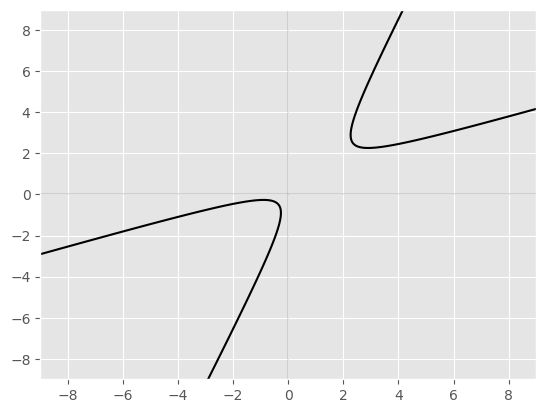
Nonstandard hyperbola#
The general quadratic in two variables \(x,y\)
\( Ax^2+Bxy+Cx^2+Dx+Ey+F=0 \) where \(B^2-4AC\gt0\)
Show code cell source
a=  1
b= -3
c=  1
d=  1
e=  1
f=  1
assert b**2 - 4*a*c > 0

g = a*x**2 + b*x*y + c*y**2 + d*x + e*y + f

axes()
plt.contour(x,y,g,[0],colors='k');
Resources#
[P] Mas, Modesto. (21 Apr 2016). “Drawing conics in matplotlib”.