Sequences & Series#
Revised
26 Mar 2023
Imports & Environment#
Show code cell source
import numpy             as np
import pandas            as pd
import matplotlib        as mpl
import matplotlib.pyplot as plt
from   matplotlib           import gridspec
from   mpl_toolkits.mplot3d import axes3d
from   ipywidgets           import interactive
plt.style.use('ggplot');

import sympy as smp
from   sympy import *

import plotly
import plotly.figure_factory as ff
import plotly.graph_objects  as go

from IPython.display import display, Math

from   datetime import datetime as d
import locale                   as l
import platform                 as p
import sys                      as s

pad = 20
print(f"{'Executed'.upper():<{pad}}: {d.now()}")
print()
print(f"{'Platform'        :<{pad}}: "
      f"{p.mac_ver()[0]} | "
      f"{p.system()} | "
      f"{p.release()} | "
      f"{p.machine()}")
print(f"{''                :<{pad}}: {l.getpreferredencoding()}")
print()
print(f"{'Python'          :<{pad}}: {s.version}")
print(f"{''                :<{pad}}: {s.version_info}")
print(f"{''                :<{pad}}: {p.python_implementation()}")
print()
print(f"{'Matplotlib'      :<{pad}}: {mpl   .__version__}")
print(f"{'NumPy'           :<{pad}}: {np    .__version__}")
print(f"{'Pandas'          :<{pad}}: {pd    .__version__}")
print(f"{'Plotly'          :<{pad}}: {plotly.__version__}")
print(f"{'SymPy'           :<{pad}}: {smp   .__version__}")
EXECUTED            : 2024-10-28 14:22:29.215869

Platform            : 15.1 | Darwin | 24.1.0 | arm64
                    : UTF-8

Python              : 3.11.9 | packaged by conda-forge | (main, Apr 19 2024, 18:34:54) [Clang 16.0.6 ]
                    : sys.version_info(major=3, minor=11, micro=9, releaselevel='final', serial=0)
                    : CPython

Matplotlib          : 3.8.4
NumPy               : 1.26.4
Pandas              : 2.2.2
Plotly              : 5.22.0
SymPy               : 1.12
Sequences#
Sequences as functions#
A infinite sequence can be thought of as a list of numbers written in a definite order
\( \begin{aligned} \{a_n\}_{n=1}^\infty \overset{\text{def}}{=} a_1,a_2,a_3,...,a_n,... \end{aligned} \)
where \(a_1\) is the first term, \(a_2\) is the second term, and in general \(a_n\) is the \(n\)-th term.
In an infinite sequence, each term \(a_n\) has a successor term \(a_{n+1}\).
For every positive integer \(n\) there is a corresponding number \(a_n\). Therefore, a sequence can be defined as a function \(f\) whose domain is the set of positive integers and where \(a_n\) denotes the value of the function at the number \(n\).
\( \begin{aligned} \{a_n\}_{n=1}^\infty \overset{\text{def}}{=} f:n\mapsto a_n \,\,\,\text{where}\,n\in\mathbb{Z}^+ \end{aligned} \)
Graph of a Sequence#
Since a sequence is a function whose domain is the set of positive integers, its graph consists of isolated points with coordinates
\( (1,a_1),(2,a_2),(3,a_3),...,(n,a_n),... \)
Limit of a Sequence#
Convergence and Divergence#
A sequence is said to converge if the limit \(L\) of the sequence exists.
A sequence is said to diverge if the limit \(L\) of the sequence doesn’t exists.
Convergent Sequence#
The notation
\( \begin{aligned} \lim_{n\to\infty}a_n=L \end{aligned} \)
or
\( a_n\to L \,\,\,\text{as}\,\,\, n\to\infty \)
means that the terms of the sequence \(\{a_n\}\) approach \(L\) as \(n\) becomes large.
In other words, a sequence \(\{a_n\}\) has the limit \(L\) if we can make the terms \(a_n\) arbitrarily close to \(L\) by taking \(n\) sufficiently large.
More precisely, a sequence \(\{a_n\}\) has the limit \(L\) if for every \(\varepsilon\gt0\) there is a corresponding integer \(N\) such that if \(n\gt N\) then \(|a_n-L|\lt\varepsilon\)
Sequence Diverging to Infinity#
The notation
\( \begin{aligned} \lim_{n\to\infty}a_n=\infty \end{aligned} \)
means that if \(a_n\) becomes large as \(n\) becomes large. (In other words, the sequence \(\{a_n\}\) diverges to infinity.)
More precisely, this means that for every positive number \(M\) there is an integer \(N\) such that if \(n\gt N\) then \(a_n\gt M\).
Limit Laws for Sequences#
Let \(\{a_n\}\) and \(\{b_n\}\) be convergent sequences and \(c\) be a constant.
\( \begin{aligned} \lim_{n\to\infty}(a_n\pm b_n)=\lim_{n\to\infty}a_n\pm\lim_{n\to\infty}b_n \end{aligned} \)
\( \begin{aligned} \lim_{n\to\infty}ca_n=c\lim_{n\to\infty}a_n \end{aligned} \)
\( \begin{aligned} \lim_{n\to\infty}c=c \end{aligned} \)
\( \begin{aligned} \lim_{n\to\infty}(a_nb_n)=\lim_{n\to\infty}a_n\cdot\lim_{n\to\infty}b_n \end{aligned} \)
\( \begin{aligned} \lim_{n\to\infty}\left(\frac{a_n}{b_n}\right)=\frac{\begin{aligned}\lim_{n\to\infty}a_n\end{aligned}}{\begin{aligned}\lim_{n\to\infty}b_n\end{aligned}} \,\,\,\text{if}\,\lim_{n\to\infty}b_n\ne0 \end{aligned} \)
\( \begin{aligned} \lim_{n\to\infty}a_n^p=\left[\lim_{n\to\infty}a_n\right]^p \,\,\,\text{if}\,p\gt0,a_n\gt0 \end{aligned} \)
Squeeze Theorem for Sequences#
\( \begin{aligned} a_n\le b_n\le c_n \,\,\,\text{for}\,n\ge n_0 \\ \land \\ \lim_{n\to\infty}a_n=\lim_{n\to\infty}c_n=L \\ \implies \\ \lim_{n\to\infty}b_n=L \end{aligned} \)
Theorem#
If
\( \begin{aligned} \lim_{x\to\infty}f(x)=L \end{aligned} \)
and \(f(n)=a_n\) when \(n\) is an integer, then
\( \begin{aligned} \lim_{n\to\infty}a_n=L \end{aligned} \)
Since
\( \begin{aligned} \lim_{x\to\infty}\frac{1}{x^r}=0 \,\,\,\text{when}\,r\gt0 \end{aligned} \)
it follows that
\( \begin{aligned} \lim_{n\to\infty}\frac{1}{n^r}=0 \,\,\,\text{when}\,r\gt0 \end{aligned} \)
Theorem#
\( \begin{aligned} \lim_{n\to\infty}|a_n|=0 \implies \lim_{n\to\infty}a_n=0 \end{aligned} \)
Theorem#
If
\( \begin{aligned} \lim_{n\to\infty}a_n=L \end{aligned} \)
and the function \(f\) is continuous at \(L\), then
\( \begin{aligned} \lim_{n\to\infty}f(a_n)=f(L) \end{aligned} \)
That is, if we apply a continuous function to the terms of a convergent sequence, the result is also convergent.
Monotonicity of Sequences#
A sequence \(\{a_n\}\) is called increasing if \(a_n\lt a_{n+1}\) for all \(n\ge1\). That is, \(a_1\lt a_2\lt a_3\lt...\).
A sequence \(\{a_n\}\) is called decreasing if \(a_n\gt a_{n+1}\) for all \(n\ge1\). That is, \(a_1\gt a_2\gt a_3\gt...\).
A sequence is called monotonic if it is either increasing or decreasing.
\(\begin{aligned}\{r^n\}\end{aligned}\)#
The sequence
\( \begin{aligned} \{r^n\} \end{aligned} \)
converges if \(-1\lt r\le1\) and diverges otherwise.
\( \begin{aligned} \lim_{n\to\infty}\{r^n\}= \begin{cases} \infty &\text{if}\,\,\, r\gt1 \\ 1 &\text{if}\,\,\, r=1 \\ 0 &\text{if}\,\,\, -1\lt r\lt1 \\ \text{DNE} &\text{if}\,\,\, r\le-1 \end{cases} \end{aligned} \)
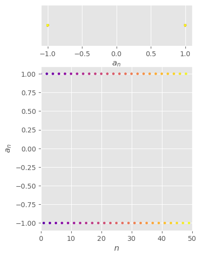
\(r=-1\)#
\( \begin{aligned} \{(-1)^n\}_{n=1}^\infty =\{-1,1,-1,1,-1,1,...,(-1)^n,...\} \end{aligned} \)
divergent
\( \begin{aligned} \lim_{n\to\infty}(-1)^n=\text{DNE} \end{aligned} \)
bounded
\( -1\le(-1)^n\le1 \,\,\,\forall n\ge1 \)
Show code cell source
def seq ():
  n=1
  while True:
    yield (-1)**n
    n+=1
s=seq()
x,y=[range(-9,50)],[next(s) for _ in range(-9,50)]

fig,(ax1,ax2)=plt.subplots(2,1,figsize=(4,6),height_ratios=[1,4]);

ax1.scatter(y, np.zeros(59), c=x, cmap='plasma', s=10);
ax1.set_xlim(-1.1,1.1);
ax1.set_xlabel('$a_n$');
ax1.set_yticks([]);
ax1.set_ylim(-1,1);

ax2.set_xlim(0,50);
ax2.set_xlabel('$n$');
ax2.set_ylim(-1.1,1.1);
ax2.set_ylabel('$a_n$');
ax2.scatter(x, y, c=x, cmap='plasma', s=10);
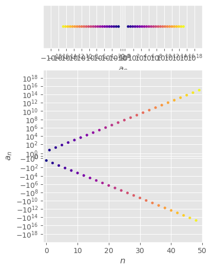
\(r=-2\)#
\( \begin{aligned} \{(-2)^n\}_{n=1}^\infty =\{-2,4,-8,16,-32,64,...,(-2)^n,...\} \end{aligned} \)
divergent
\( \begin{aligned} \lim_{n\to\infty}(-2)^n=\text{DNE} \end{aligned} \)
unbounded
Show code cell source
def seq ():
  n=1
  while True:
    yield (-2)**n
    n+=1
s=seq()
x,y=[range(0,50)],[next(s) for _ in range(0,50)]

fig,(ax1,ax2)=plt.subplots(2,1,figsize=(4,6),height_ratios=[1,4]);

ax1.scatter(y, np.zeros(50), c=x, cmap='plasma', s=10);
ax1.set_xscale('symlog');
ax1.set_xlim(-1e20,1e20);
ax1.set_xlabel('$a_n$');
ax1.set_yticks([]);
ax1.set_ylim(-1,1);

ax2.set_xlim(-1,50);
ax2.set_xlabel('$n$');
ax2.set_yscale('symlog');
ax2.set_ylim(-1e20,1e20);
ax2.set_ylabel('$a_n$');
ax2.scatter(x, y, c=x, cmap='plasma', s=10);
Boundedness of Sequences#
A sequence \(\{a_n\}\) is bounded above if there is a number \(M\) such that \(a_n\le M\) for all \(n\ge1\).
A sequence \(\{a_n\}\) is bounded below if there is a number \(m\) such that \(m\le a_n\) for all \(n\ge1\).
If it is bounded above and below, then \(\{a_n\}\) is a bounded sequence.
Completeness Axiom for the set of real numbers \(\mathbb{R}\)#
If \(S\) is a nonempty set of real numbers that has an upper bound \(M\) such that
\(x\le M\,\,\,\forall x\in S\)
then \(S\) has a least upper bound \(b\).
This means that \(b\) is an upper bound for \(S\), but if \(M\) is any other upper bound, then \(b\le M\).
If \(S\) is a nonempty set of real numbers that has a lower bound \(m\) such that
\(m\le x\,\,\,\forall x\in S\)
then \(S\) has a greatest lower bound \(B\).
This means that \(B\) is a lower bound for \(S\), but if \(m\) is any other lower bound, then \(B\ge m\).
In other words, there is no gap or hole in the real number line.
Monotonic Sequence Theorem#
Not every bounded sequence is convergent.
Not every monotonic sequence is convergent.
Monotonic Sequence Theorem: Every bounded, monotonic sequence is convergent.
(Any increasing sequence that is bounded above is convergent; and decreasing sequence that is bounded below is convergent.)
PROOF
Let \(\{a_n\}\) be an increasing sequence.
Since \(\{a_n\}\) is bounded, the set \(S=\{a_n\mid n\ge1\}\) has an upper bound; and by the Completeness Axiom, it has a least upper bound \(L\).
Given \(\varepsilon\gt0\), \(L-\varepsilon\) is not an upper bound for \(S\) since \(L\) is the least upper bound.
Thus, \(a_N\gt L-\varepsilon\) for some integer \(N\).
But the sequence is increasing, so \(a_n\ge a_N\) for every \(n\gt N\).
Thus, if \(n\gt N\), then \(a_n\gt L-\varepsilon\), so \(0\le L-a_n\le\varepsilon\) since \(a_n\le L\).
Thus, \(|L-a_n|\lt\varepsilon\) when \(n\gt N\).
Therefore, \(\begin{aligned}\lim_{n\to\infty}a_n=L\end{aligned}\)
\(\blacksquare\)
Examples of Sequences#
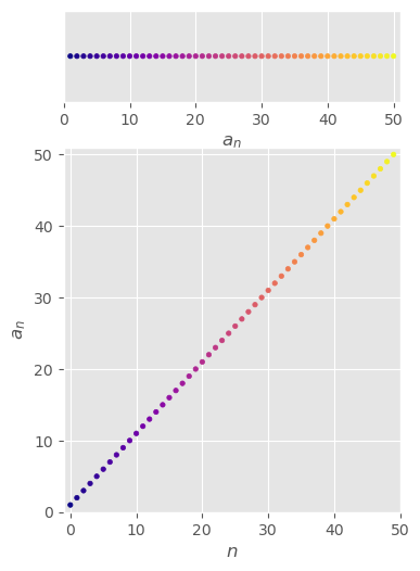
\(\{n\}_{n=1}^\infty\)#
\( \{n\}_{n=1}^\infty =\{1,2,3,4,5,...,n,...\} \)
divergent to infinity
\( \begin{aligned} \lim_{n\to\infty}n=\infty \end{aligned} \)
monotonically increasing
\( (n+1)=a_{n+1}\gt a_n=n \)
bounded from below
\( 1\le a_{n} \,\,\,\forall n\ge1 \)
Show code cell source
def seq ():
  n=1
  while True:
    yield n
    n+=1
s=seq()
x,y=[range(50)],[next(s) for _ in range(50)]

fig,(ax1,ax2)=plt.subplots(2,1,figsize=(4,6),height_ratios=[1,4]);

ax1.scatter(y, np.zeros(50), c=x, cmap='plasma', s=10);
ax1.set_xlim(0,51);
ax1.set_xlabel('$a_n$');
ax1.set_yticks([]);
ax1.set_ylim(-1,1);

ax2.set_xlim(-1,50);
ax2.set_xlabel('$n$');
ax2.set_ylim(0,51);
ax2.set_ylabel('$a_n$');
ax2.scatter(x, y, c=x, cmap='plasma', s=10);
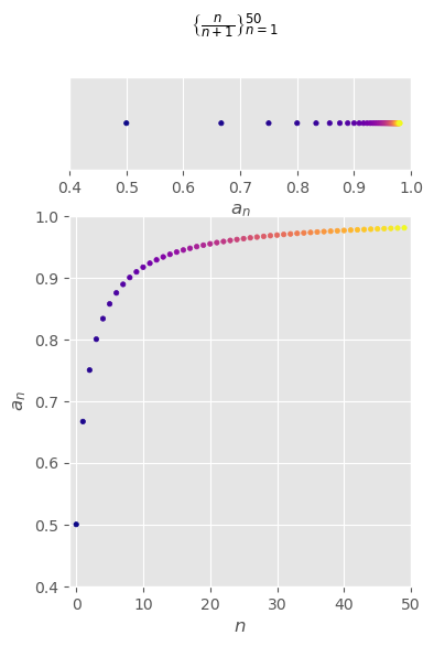
\(\begin{aligned}\left\{\frac{n}{n+1}\right\}_{n=1}^\infty\end{aligned}\)#
\( \begin{aligned} \left\{\frac{n}{n+1}\right\}_{n=1}^\infty =\left\{\frac{1}{2},\frac{2}{3},\frac{3}{4},\frac{4}{5},\frac{5}{6},...,\frac{n}{n+1},...\right\} \end{aligned} \)
convergent
\( \begin{aligned} \lim_{n\to\infty}\frac{n}{n+1} =\lim_{n\to\infty}\frac{1}{1+\frac{1}{n}} =\frac{\begin{aligned}\lim_{n\to\infty}1\end{aligned}}{\begin{aligned}\lim_{n\to\infty}1+\lim_{n\to\infty}\frac{1}{n}\end{aligned}} =\frac{1}{1+0} =1 \end{aligned} \)
monotonically increasing
\( \begin{aligned} \frac{n}{n+1}=a_n\lt a_{n+1}=\frac{(n+1)}{(n+1)+1}=\frac{n+1}{n+2} \end{aligned} \)
bounded
\( \begin{aligned} \frac{1}{2}\le\frac{n}{n+1}\le1 \,\,\,\forall n\ge1 \end{aligned} \)
Show code cell source
def seq ():
  n=1
  while True:
    yield n/(n+1)
    n+=1
s=seq()
x,y=[range(50)],[next(s) for _ in range(50)]

fig,(ax1,ax2)=plt.subplots(2,1,figsize=(4,6),height_ratios=[1,4]);

ax1.scatter(y, np.zeros(50), c=x, cmap='plasma', s=10);
ax1.set_xlim(0.4, 1);
ax1.set_xlabel('$a_n$');
ax1.set_yticks([]);
ax1.set_ylim(-1,1);

ax2.set_xlim(-1 ,50);
ax2.set_xlabel('$n$');
ax2.set_ylim(0.4, 1);
ax2.set_ylabel('$a_n$');
ax2.scatter(x, y, c=x, cmap='plasma', s=10);

fig.suptitle('$\\left\\{\\frac{n}{n+1}\\right\\}_{n=1}^{50}$');
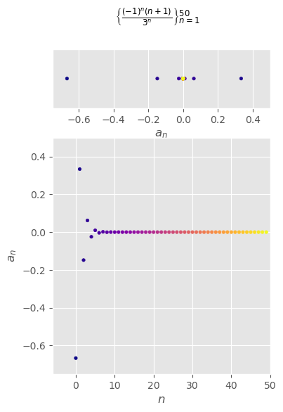
\(\begin{aligned}\left\{\frac{(-1)^n(n+1)}{3^n}\right\}_{n=1}^\infty\end{aligned}\)#
\( \begin{aligned} \left\{\frac{(-1)^n(n+1)}{3^n}\right\}_{n=1}^\infty =\left\{-\frac{2}{3},\frac{3}{9},-\frac{4}{27},\frac{5}{81},...,\frac{(-1)^n(n+1)}{3^n},...\right\} \end{aligned} \)
Show code cell source
def seq ():
  n=1
  while True:
    yield (-1)**n*(n+1)/3**n
    n+=1
s=seq()
x,y=[range(50)],[next(s) for _ in range(50)]

fig,(ax1,ax2)=plt.subplots(2,1,figsize=(4,6),height_ratios=[1,4]);

ax1.scatter(y, np.zeros(50), c=x, cmap='plasma', s=10);
ax1.set_xlim(-0.75, 0.5);
ax1.set_xlabel('$a_n$');
ax1.set_yticks([]);
ax1.set_ylim(-1,1);

ax2.set_xlim(-6 ,50);
ax2.set_xlabel('$n$');
ax2.set_ylim(-0.75, 0.5);
ax2.set_ylabel('$a_n$');
ax2.scatter(x, y, c=x, cmap='plasma', s=10);

fig.suptitle('$\\left\\{\\frac{(-1)^n(n+1)}{3^n}\\right\\}_{n=1}^{50}$');
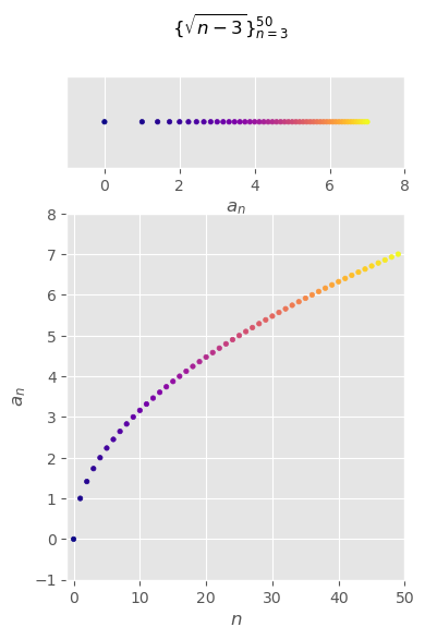
\(\begin{aligned}\{\sqrt{n-3}\}_{n=3}^\infty\end{aligned}\)#
\( \begin{aligned} \{\sqrt{n-3}\}_{n=3}^\infty =\left\{0,1,\sqrt{2},\sqrt{3},...,\sqrt{n-3},...\right\} \end{aligned} \)
Show code cell source
def seq ():
  n=3
  while True:
    yield np.sqrt(n-3)
    n+=1
s=seq()
x,y=[range(50)],[next(s) for _ in range(50)]

fig,(ax1,ax2)=plt.subplots(2,1,figsize=(4,6),height_ratios=[1,4]);

ax1.scatter(y, np.zeros(50), c=x, cmap='plasma', s=10);
ax1.set_xlim(-1,8);
ax1.set_xlabel('$a_n$');
ax1.set_yticks([]);
ax1.set_ylim(-1,1);

ax2.set_xlim(-1,50);
ax2.set_xlabel('$n$');
ax2.set_ylim(-1,8);
ax2.set_ylabel('$a_n$');
ax2.scatter(x, y, c=x, cmap='plasma', s=10);

fig.suptitle('$\\{\\sqrt{n-3}\\}_{n=3}^{50}$');
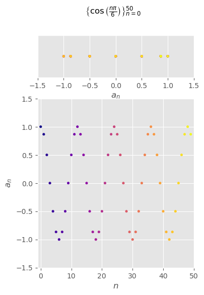
\(\begin{aligned}\left\{\cos\left(\frac{n\pi}{6}\right)\right\}_{n=0}^\infty\end{aligned}\)#
\( \begin{aligned} \left\{\cos\left(\frac{n\pi}{6}\right)\right\}_{n=0}^\infty =\left\{1,\frac{\sqrt{3}}{2},\frac{1}{2},0,...,\cos\left(\frac{n\pi}{6}\right),...\right\} \end{aligned} \)
Show code cell source
def seq ():
  n=0
  while True:
    yield np.cos(n*np.pi/6)
    n+=1
s=seq()
x,y=[range(50)],[next(s) for _ in range(50)]

fig,(ax1,ax2)=plt.subplots(2,1,figsize=(4,6),height_ratios=[1,4]);

ax1.scatter(y, np.zeros(50), c=x, cmap='plasma', s=10);
ax1.set_xlim(-1.5,1.5);
ax1.set_xlabel('$a_n$');
ax1.set_yticks([]);
ax1.set_ylim(-1,1);

ax2.set_xlim(-1,50);
ax2.set_xlabel('$n$');
ax2.set_ylim(-1.5,1.5);
ax2.set_ylabel('$a_n$');
ax2.scatter(x, y, c=x, cmap='plasma', s=10);

fig.suptitle('$\\left\\{\\cos\\left(\\frac{n\\pi}{6}\\right)\\right\\}_{n=0}^{50}$');
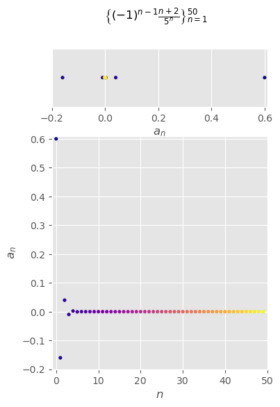
\(\begin{aligned}\left\{(-1)^{n-1}\frac{n+2}{5^n}\right\}_{n=1}^\infty\end{aligned}\)#
\( \begin{aligned} \left\{(-1)^{n-1}\frac{n+2}{5^n}\right\}_{n=1}^\infty =\left\{\frac{3}{5},-\frac{4}{25},\frac{5}{125},-\frac{6}{625},...,(-1)^{n-1}\frac{n+2}{5^n},...\right\} \end{aligned} \)
Show code cell source
def seq ():
  n=1
  while True:
    yield (-1)**(n-1)*((n+2)/5**n)
    n+=1
s=seq()
x,y=[range(50)],[next(s) for _ in range(50)]

fig,(ax1,ax2)=plt.subplots(2,1,figsize=(4,6),height_ratios=[1,4]);

ax1.scatter(y, np.zeros(50), c=x, cmap='plasma', s=10);
ax1.set_xlim(-0.2, 0.61);
ax1.set_xlabel('$a_n$');
ax1.set_yticks([]);
ax1.set_ylim(-1,1);

ax2.set_xlim(-1,50);
ax2.set_xlabel('$n$');
ax2.set_ylim(-0.2, 0.61);
ax2.set_ylabel('$a_n$');
ax2.scatter(x, y, c=x, cmap='plasma', s=10);

fig.suptitle('$\\left\\{(-1)^{n-1}\\frac{n+2}{5^n}\\right\\}_{n=1}^{50}$');
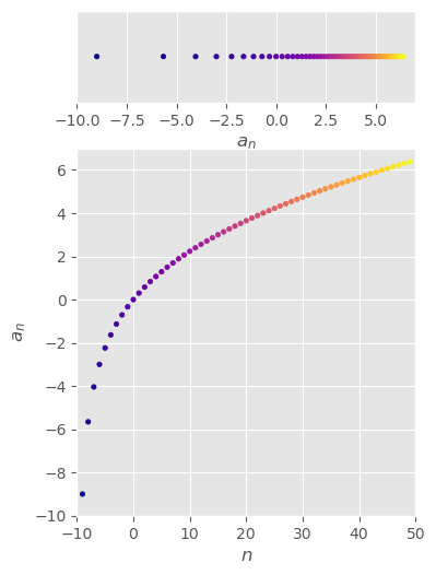
\(\begin{aligned}\left\{\frac{n}{\sqrt{10+n}}\right\}_{n=-9}^\infty\end{aligned}\)#
\( \begin{aligned} \left\{\frac{n}{\sqrt{10+n}}\right\}_{n=-9}^\infty \end{aligned} \)
divergent to infinity
\( \begin{aligned} \lim_{n\to\infty}\frac{n}{\sqrt{10+n}} =\lim_{n\to\infty}\frac{\frac{1}{n}n}{\frac{1}{n}\sqrt{10+n}} =\lim_{n\to\infty}\frac{1}{\sqrt{\frac{10}{n^2}+\frac{1}{n}}} =\infty \end{aligned} \)
Show code cell source
def seq ():
  n=-9
  while True:
    yield n/np.sqrt(10+n)
    n+=1
s=seq()
x,y=[range(-9,50)],[next(s) for _ in range(-9,50)]

fig,(ax1,ax2)=plt.subplots(2,1,figsize=(4,6),height_ratios=[1,4]);

ax1.scatter(y, np.zeros(59), c=x, cmap='plasma', s=10);
ax1.set_xlim(-10,7);
ax1.set_xlabel('$a_n$');
ax1.set_yticks([]);
ax1.set_ylim(-1,1);

ax2.set_xlim(-10,50);
ax2.set_xlabel('$n$');
ax2.set_ylim(-10,7);
ax2.set_ylabel('$a_n$');
ax2.scatter(x, y, c=x, cmap='plasma', s=10);
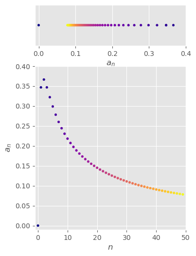
\(\begin{aligned}\left\{\frac{\ln n}{n}\right\}_{n=1}^\infty\end{aligned}\)#
\( \begin{aligned} \left\{\frac{\ln n}{n}\right\}_{n=1}^\infty \end{aligned} \)
convergent
\( \begin{aligned} &f(x)=\frac{\ln x}{x} \\ &\lim_{x\to\infty}\frac{\ln x}{x} =\lim_{x\to\infty}\frac{\frac{1}{x}}{1} \,\,\,\text{by L'Hospital's Rule} =\frac{\begin{aligned}\lim_{x\to\infty}\frac{1}{x}\end{aligned}}{\begin{aligned}\lim_{x\to\infty}1\end{aligned}} =\frac{0}{1} =0 \\ &\lim_{x\to\infty}\frac{\ln x}{x}=0 \implies \lim_{n\to\infty}\frac{\ln n}{n}=0 \,\,\,\text{by theorem} \end{aligned} \)
Show code cell source
def seq ():
  n=1
  while True:
    yield np.log(n)/n
    n+=1
s=seq()
x,y=[range(0,50)],[next(s) for _ in range(0,50)]

fig,(ax1,ax2)=plt.subplots(2,1,figsize=(4,6),height_ratios=[1,4]);

ax1.scatter(y, np.zeros(50), c=x, cmap='plasma', s=10);
ax1.set_xlim(-0.01,0.4);
ax1.set_xlabel('$a_n$');
ax1.set_yticks([]);
ax1.set_ylim(-1,1);

ax2.set_xlim(-1,50);
ax2.set_xlabel('$n$');
ax2.set_ylim(-0.01,0.4);
ax2.set_ylabel('$a_n$');
ax2.scatter(x, y, c=x, cmap='plasma', s=10);
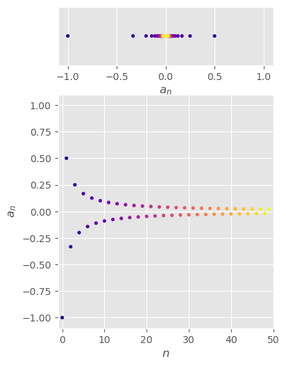
\(\begin{aligned}\left\{\frac{(-1)^n}{n}\right\}_{n=1}^\infty\end{aligned}\)#
\( \begin{aligned} \left\{\frac{(-1)^n}{n}\right\}_{n=1}^\infty =\left\{-1,\frac{1}{2},-\frac{1}{3},\frac{1}{4},-\frac{1}{5},\frac{1}{6},...,\frac{(-1)^n}{n},...\right\} \end{aligned} \)
convergent
\( \begin{aligned} &\lim_{n\to\infty}\left|\frac{(-1)^n}{n}\right| =\lim_{n\to\infty}\frac{1}{n} =0 \\ &\lim_{n\to\infty}\left|\frac{(-1)^n}{n}\right|=0 \implies \lim_{n\to\infty}\frac{(-1)^n}{n}=0 \,\,\,\text{by theorem} \end{aligned} \)
Show code cell source
def seq ():
  n=1
  while True:
    yield (-1)**n/n
    n+=1
s=seq()
x,y=[range(0,50)],[next(s) for _ in range(0,50)]

fig,(ax1,ax2)=plt.subplots(2,1,figsize=(4,6),height_ratios=[1,4]);

ax1.scatter(y, np.zeros(50), c=x, cmap='plasma', s=10);
ax1.set_xlim(-1.1,1.1);
ax1.set_xlabel('$a_n$');
ax1.set_yticks([]);
ax1.set_ylim(-1,1);

ax2.set_xlim(-1,50);
ax2.set_xlabel('$n$');
ax2.set_ylim(-1.1,1.1);
ax2.set_ylabel('$a_n$');
ax2.scatter(x, y, c=x, cmap='plasma', s=10);
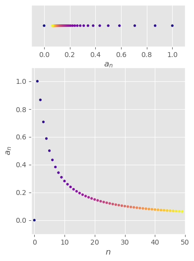
\(\begin{aligned}\left\{\sin\left(\frac{\pi}{n}\right)\right\}_{n=1}^\infty\end{aligned}\)#
\( \begin{aligned} \left\{\sin\left(\frac{\pi}{n}\right)\right\}_{n=1}^\infty \end{aligned} \)
convergent
\( \begin{aligned} \lim_{n\to\infty}\sin\left(\frac{\pi}{n}\right) =\sin\left(\pi\lim_{n\to\infty}\frac{1}{n}\right) \,\,\,\text{by theorem} =\sin(0) =0 \end{aligned} \)
Show code cell source
def seq ():
  n=1
  while True:
    yield np.sin(np.pi/n)
    n+=1
s=seq()
x,y=[range(0,50)],[next(s) for _ in range(0,50)]

fig,(ax1,ax2)=plt.subplots(2,1,figsize=(4,6),height_ratios=[1,4]);

ax1.scatter(y, np.zeros(50), c=x, cmap='plasma', s=10);
ax1.set_xlim(-0.1,1.1);
ax1.set_xlabel('$a_n$');
ax1.set_yticks([]);
ax1.set_ylim(-1,1);

ax2.set_xlim(-1,50);
ax2.set_xlabel('$n$');
ax2.set_ylim(-0.1,1.1);
ax2.set_ylabel('$a_n$');
ax2.scatter(x, y, c=x, cmap='plasma', s=10);
\(\begin{aligned}\left\{\frac{n!}{n^n}\right\}_{n=1}^\infty\end{aligned}\)#
\( \begin{aligned} \left\{\frac{n!}{n^n}\right\}_{n=1}^\infty \end{aligned} \)
convergent
\( \begin{aligned} &0\lt a_n =\frac{n!}{n^n} =\frac{1\cdot2\cdot3\cdot...\cdot n}{n\cdot n\cdot n\cdot...\cdot n} =\frac{1}{n}\left(\frac{2\cdot3\cdot...\cdot n}{n\cdot n\cdot...\cdot n}\right) \le\frac{1}{n} \,\,\,\text{since}\,2\cdot3\cdot...\cdot n\le n\cdot n\cdot...\cdot n \implies \left(\frac{2\cdot3\cdot...\cdot n}{n\cdot n\cdot...\cdot n}\right)\le1 \\ &\lim_{n\to\infty}0=0 \lt \lim_{n\to\infty}a_n \le \lim_{n\to\infty}\frac{1}{n}=0 \implies \lim_{n\to\infty}a_n=0 \,\,\,\text{by Squeeze Theorem} \end{aligned} \)
Show code cell source
def seq ():
  n=1
  while True:
    yield scipy.special.factorial(n)/n**n
    n+=1
s=seq()
x,y=[range(0,50)],[next(s) for _ in range(0,50)]

fig,(ax1,ax2)=plt.subplots(2,1,figsize=(4,6),height_ratios=[1,4]);

ax1.scatter(y, np.zeros(50), c=x, cmap='plasma', s=10);
ax1.set_xlim(-0.1,1.1);
ax1.set_xlabel('$a_n$');
ax1.set_yticks([]);
ax1.set_ylim(-1,1);

ax2.set_xlim(-1,50);
ax2.set_xlabel('$n$');
ax2.set_ylim(-0.1,1.1);
ax2.set_ylabel('$a_n$');
ax2.scatter(x, y, c=x, cmap='plasma', s=10);
---------------------------------------------------------------------------
NameError                                 Traceback (most recent call last)
Cell In[14], line 7
      5     n+=1
      6 s=seq()
----> 7 x,y=[range(0,50)],[next(s) for _ in range(0,50)]
      9 fig,(ax1,ax2)=plt.subplots(2,1,figsize=(4,6),height_ratios=[1,4]);
     11 ax1.scatter(y, np.zeros(50), c=x, cmap='plasma', s=10);

Cell In[14], line 7, in <listcomp>(.0)
      5     n+=1
      6 s=seq()
----> 7 x,y=[range(0,50)],[next(s) for _ in range(0,50)]
      9 fig,(ax1,ax2)=plt.subplots(2,1,figsize=(4,6),height_ratios=[1,4]);
     11 ax1.scatter(y, np.zeros(50), c=x, cmap='plasma', s=10);

Cell In[14], line 4, in seq()
      2 n=1
      3 while True:
----> 4   yield scipy.special.factorial(n)/n**n
      5   n+=1

NameError: name 'scipy' is not defined
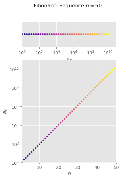
Fibonacci Sequence#
\( \{f_n\} =\begin{cases} f_1\overset{\text{def}}{=}1 \\ f_2\overset{\text{def}}{=}1 \\ f_n=f_{n-1}+f_{n-2} \,\,\,\text{when}\,n\ge3 \end{cases} =\{1,1,2,3,5,8,13,21,...\} \)
Show code cell source
def seq (n):
  a, b = 1, 1
  for _ in range(n):
    yield a
    a, b = b, a + b
s=seq(50)
x,y=[range(50)],[next(s) for _ in range(50)]

fig,(ax1,ax2)=plt.subplots(2,1,figsize=(4,6),height_ratios=[1,4]);

ax1.scatter(y, np.zeros(50), c=x, cmap='plasma', s=10);
ax1.set_xscale('log');
ax1.set_xlim(1, 1e11);
ax1.set_xlabel('$a_n$');
ax1.set_yticks([]);
ax1.set_ylim(-1,1);

ax2.set_xlim(1,50);
ax2.set_xlabel('$n$');
ax2.set_yscale('log');
ax2.set_ylim(1,1e11);
ax2.set_ylabel('$a_n$');
ax2.scatter(x, y, c=x, cmap='plasma', s=10);

fig.suptitle('Fibonacci Sequence $n=50$');
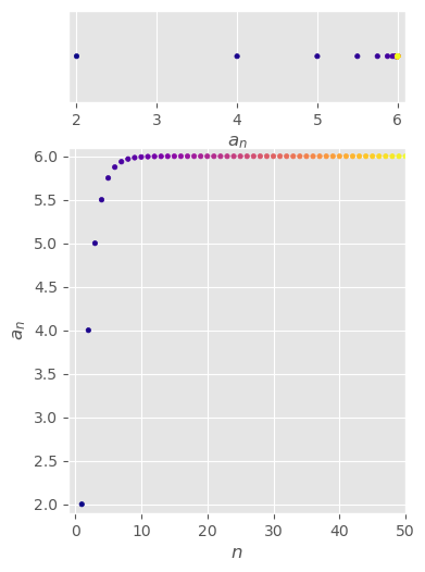
\(\begin{aligned}\{a_n\}_{n=1}^\infty=\begin{cases}a_1&=2\\a_{n+1}&=\frac{1}{2}(a_n+6)\end{cases}\end{aligned}\)#
\( \begin{aligned} \{a_n\}_{n=1}^\infty= \begin{cases} a_1&=2 \\ a_{n+1}&=\frac{1}{2}(a_n+6) \end{cases} =\left\{2,4,5,\frac{11}{2},\frac{23}{4},\frac{47}{8},...\right\} \end{aligned} \)
monotonically increasing
\( a_{n+1}\gt a_n \,\,\,\forall n\ge1 \,\,\,\text{by induction} \\ a_{n+1}\gt a_n \,\,\,\text{when}\,n=1 \,\,\,\text{since}\,4=a_2\gt a_1=2 \\ a_{n+1}\gt a_n \,\,\,\text{when}\,n=k \,\,\,\text{assumed by induction hypothesis} \\ a_{k+1}\gt a_k \iff a_{k+1}+6\gt a_k+6 \iff \frac{1}{2}(a_{k+1}+6)\gt\frac{1}{2}(a_{k}+6) \\ \implies a_{k+2}\gt a_{k+1} \\ a_{n+1}\gt a_n \,\,\,\text{when}\,n=k+1 \)
bounded
\( 2\le a_n\lt6 \,\,\,\forall n\ge1 \,\,\,\text{by induction} \\ 2\le a_n\lt6 \,\,\,\text{when}\,n=1 \,\,\,\text{since}\,a_1=2\lt6 \\ 2\le a_n\lt6 \,\,\,\text{when}\,n=k \,\,\,\text{assumed by induction hypothesis} \\ a_k\lt6 \iff a_k+6\lt12 \iff \frac{1}{2}(a_k+6)\lt6 \\ \implies a_{k+1}\lt 6 \\ 2\le a_n\lt6 \,\,\,\text{when}\,n=k+1 \)
convergent
\( \begin{aligned} \lim_{n\to\infty}a_n=L \implies \lim_{n\to\infty}a_{n+1}=L \,\,\,\text{since}\,\,\, n\to\infty \implies n+1\to\infty \end{aligned} \)
\( \begin{aligned} L =\lim_{n\to\infty}a_{n+1} =\lim_{n\to\infty}\frac{1}{2}(a_n+6) =\frac{1}{2}(\lim_{n\to\infty}a_n+6) =\frac{1}{2}(L+6) \\ L=\frac{1}{2}(L+6) \implies L=\frac{1}{2}L+3 \implies L=6 \end{aligned} \)
Show code cell source
def seq (n):
  a, b = 2, 4
  for _ in range(n):
    yield a
    a, b = b, (1/2)*(b+6)
s=seq(50)
x,y=[range(1,51)],[next(s) for _ in range(1,51)]

fig,(ax1,ax2)=plt.subplots(2,1,figsize=(4,6),height_ratios=[1,4]);

ax1.scatter(y, np.zeros(50), c=x, cmap='plasma', s=10);
ax1.set_xlim(1.9, 6.1);
ax1.set_xlabel('$a_n$');
ax1.set_yticks([]);
ax1.set_ylim(-1,1);

ax2.set_xlim(-1,50);
ax2.set_xlabel('$n$');
ax2.set_ylim(1.9,6.1);
ax2.set_ylabel('$a_n$');
ax2.scatter(x, y, c=x, cmap='plasma', s=10);
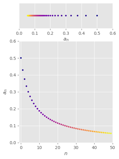
\(\begin{aligned}\left\{\frac{3}{n+5}\right\}_{n=1}^\infty\end{aligned}\)#
\( \begin{aligned} \left\{\frac{3}{n+5}\right\}_{n=1}^\infty =\left\{\frac{1}{2},\frac{3}{7},\frac{3}{8},\frac{1}{3},\frac{3}{10},\frac{3}{11},...,\frac{3}{n+5},...\right\} \end{aligned} \)
convergent
\( \begin{aligned} \lim_{n\to\infty}0=0 \lt 3\lim_{n\to\infty}\frac{1}{n+5} \lt 3\lim_{n\to\infty}\frac{1}{n}=0 \implies \lim_{n\to\infty}\frac{3}{n+5}=0 \,\,\,\text{by Squeeze Theorem} \end{aligned} \)
monotonically decreasing
\( \begin{aligned} \frac{3}{n+5}=a_n\gt a_{n+1}=\frac{3}{(n+1)+5}=\frac{3}{n+6} \end{aligned} \)
Show code cell source
def seq ():
  n=1
  while True:
    yield 3/(n+5)
    n+=1
s=seq()
x,y=[range(0,50)],[next(s) for _ in range(0,50)]

fig,(ax1,ax2)=plt.subplots(2,1,figsize=(4,6),height_ratios=[1,4]);

ax1.scatter(y, np.zeros(50), c=x, cmap='plasma', s=10);
ax1.set_xlim(0,0.6);
ax1.set_xlabel('$a_n$');
ax1.set_yticks([]);
ax1.set_ylim(-1,1);

ax2.set_xlim(-1,50);
ax2.set_xlabel('$n$');
ax2.set_ylim(0,0.6);
ax2.set_ylabel('$a_n$');
ax2.scatter(x, y, c=x, cmap='plasma', s=10);
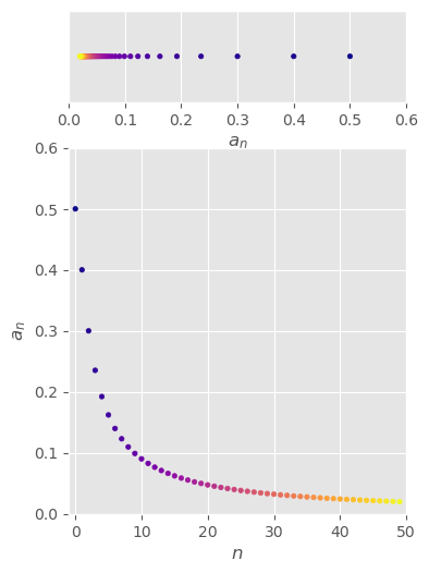
\(\begin{aligned}\left\{\frac{n}{n^2+1}\right\}_{n=1}^\infty\end{aligned}\)#
[EXAMPLE]
\( \begin{aligned} \left\{\frac{n}{n^2+1}\right\}_{n=1}^\infty =\left\{\frac{1}{2},\frac{2}{5},\frac{3}{10},\frac{4}{17},\frac{5}{26},\frac{6}{37},...,\frac{n}{n^2+1},...\right\} \end{aligned} \)
convergent
\( \begin{aligned} \lim_{n\to\infty}\frac{n}{n^2+1} =\lim_{n\to\infty}\frac{\frac{1}{n^2}n}{\frac{1}{n^2}(n^2+1)} =\lim_{n\to\infty}\frac{\frac{1}{n}}{1+\frac{1}{n^2}} =\frac{\begin{aligned}\lim_{n\to\infty}\frac{1}{n}\end{aligned}}{\begin{aligned}\lim_{n\to\infty}1+\lim_{n\to\infty}\frac{1}{n^2}\end{aligned}} =\frac{0}{1+0} =0 \end{aligned} \)
monotonically decreasing
\( \begin{aligned} \frac{(n+1)}{(n+1)^2+1}=a_{n+1}\lt a_n=\frac{n}{n^2+1} \iff (n+1)(n^2+1)\lt n((n+1)^2+1) \iff n^3+n^2+n+1\lt n^3+2n^2+2n \iff 1\lt n^2+n \,\,\,\text{for}\, n\ge1 \end{aligned} \)
or
\( \begin{aligned} f(x)=\frac{x}{x^2+1} \implies f'(x)=\frac{x^2+1-2x^2}{(x^2+1)^2} =\frac{1-x^2}{(x^2+1)^2} \lt0 \,\,\,\text{when}\, x^2\gt1 \end{aligned} \)
\(f\) is decreasing on the open interval \((1,\infty)\) and so \(f(n)\gt f(n+1)\), and so \(\{a_n\}\) is decreasing
Show code cell source
def seq ():
  n=1
  while True:
    yield n/(n**2+1)
    n+=1
s=seq()
x,y=[range(0,50)],[next(s) for _ in range(0,50)]

fig,(ax1,ax2)=plt.subplots(2,1,figsize=(4,6),height_ratios=[1,4]);

ax1.scatter(y, np.zeros(50), c=x, cmap='plasma', s=10);
ax1.set_xlim(0,0.6);
ax1.set_xlabel('$a_n$');
ax1.set_yticks([]);
ax1.set_ylim(-1,1);

ax2.set_xlim(-1,50);
ax2.set_xlabel('$n$');
ax2.set_ylim(0,0.6);
ax2.set_ylabel('$a_n$');
ax2.scatter(x, y, c=x, cmap='plasma', s=10);
Series#
Grandi’s Series#
\( \begin{aligned} \sum_{n=0}^\infty(-1)^n =1-1+1-1+1-1+1-1+... \end{aligned} \)
Arithmetic#
Arithmetic Sequence#
\( \{a,a+d,a+2d,a+3d,...\} \)
\(a\) is the sequence’s initial value
\(d\) is the common difference
\( a_n=a+(n-1)d \) is the \(n\)-th term of an arithmetic sequence
Each term is the arithmetic mean of its neighboring terms.
Arithmetic Series#
\( \begin{aligned} \sum_{k=0}^{n}a+kd =a+(a+d)+(a+2d)+(a+3d)+... \end{aligned} \)
Geometric#
Geometric Sequence#
\( \begin{aligned} \{a,ar,ar^2,ar^3,...\} \end{aligned} \)
\( a_n=ar^{n-1} \) is the \(n\)-th term of a geometric sequence
\(r\ne0\) is the common ratio
\(a\ne0\) is a scale factor equal to the sequence’s initial value
Each term is the geometric mean of its neighboring terms.
[EXAMPLE]
\( \begin{aligned} a&=1\\ r&=-3\\ \end{aligned} \)
\( \begin{aligned} \{1,-3,9,-27,81,-243,...\} =\{(1),(1)(-3),(1)(-3)^2,(1)(-3)^3,(1)(-3)^4,(1)(-3)^5,...\} \end{aligned} \)
[EXAMPLE]
\( \begin{aligned} a&=\frac{1}{2}\\ r&=\frac{1}{2}\\ \end{aligned} \)
\( \begin{aligned} &\left\{\left(\frac{1}{2}\right),\left(\frac{1}{4}\right),\left(\frac{1}{8}\right),\left(\frac{1}{16}\right),\left(\frac{1}{32}\right),\left(\frac{1}{64}\right),...\right\}\\ &=\left\{\left(\frac{1}{2}\right),\left(\frac{1}{2^2}\right),\left(\frac{1}{2^3}\right),\left(\frac{1}{2^4}\right),\left(\frac{1}{2^5}\right),\left(\frac{1}{2^6}\right),...\right\}\\ &=\left\{\left(\frac{1}{2}\right),\left(\frac{1}{2}\right)\left(\frac{1}{2}\right),\left(\frac{1}{2}\right)\left(\frac{1}{2}\right)^2,\left(\frac{1}{2}\right)\left(\frac{1}{2}\right)^3,\left(\frac{1}{2}\right)\left(\frac{1}{2}\right)^4,\left(\frac{1}{2}\right)\left(\frac{1}{2}\right)^5,...\right\} \end{aligned} \)
Geometric Series#
Generator Form
\( \begin{aligned} \sum_{k=0}^\infty ar^k =a+ar+ar^2+ar^3+... \end{aligned} \)
Closed Form
\( \begin{aligned} \frac{a}{1-r} \end{aligned} \) for \(|r|\lt1\)
[EXAMPLE]
\( \begin{aligned} &\sum_{k=0}^\infty\left(\frac{1}{2}\right)\left(\frac{1}{2}\right)^k \\ &=\frac{1}{2}+\frac{1}{4}+\frac{1}{8}+\frac{1}{16}+\frac{1}{32}+\frac{1}{64}+... \\ &=\frac{\frac{1}{2}}{1-\frac{1}{2}} \\ &=1 \end{aligned} \)
Harmonic#
Harmonic Sequence#
Harmonic Series#
\( \begin{aligned} \sum_{n=1}^\infty\frac{1}{n} =1+\frac{1}{2}+\frac{1}{3}+\frac{1}{4}+\frac{1}{5}+\frac{1}{6}+\frac{1}{7}+\frac{1}{8}+... \end{aligned} \)
Taylor Series#
\( \begin{aligned} e^x &=1+x+\frac{x^2}{2!}+\frac{x^3}{3!}+\frac{x^4}{4!}+\frac{x^5}{5!}+\frac{x^6}{6!}+\frac{x^7}{7!}+\frac{x^8}{8!}+\frac{x^9}{9!}+... \\ \sin x &=x-\frac{x^3}{3!}+\frac{x^5}{5!}-\frac{x^7}{7!}+\frac{x^9}{9!}-... \\ \cos x &=1-\frac{x^2}{2!}+\frac{x^4}{4!}-\frac{x^6}{6!}+\frac{x^8}{8!}-... \end{aligned} \)
\(\begin{aligned}8=\sum_{n=0}^\infty \frac{6}{4^n}\end{aligned}\)#
\( \begin{aligned} 8 =\sum_{n=0}^\infty \frac{6}{4^n} \end{aligned} \)
n = smp.symbols('n')

smp.Sum(6/4**n, (n, 0, smp.oo)).doit() # symbolic solution
\(\begin{aligned}\frac{10}{3}=\sum_{n=0}^\infty \frac{2^{n + 1}}{5^n}\end{aligned}\)#
\( \begin{aligned} \frac{10}{3} =\sum_{n=0}^\infty \frac{2^{n + 1}}{5^n} \end{aligned} \)
n = smp.symbols('n')

smp.Sum(2**(n + 1) / 5**n, (n, 0, smp.oo)).doit() # symbolic solution
\(\begin{aligned}15\approx\sum_{n=1}^\infty \frac{\tan^{-1}(n)}{n^{1.1}}\end{aligned}\)#
\( \begin{aligned} 15\approx \sum_{n=1}^\infty \frac{\tan^{-1}(n)}{n^{1.1}} \end{aligned} \)
n = smp.symbols('n')

smp.Sum(smp.atan(n)/n**smp.Rational(11, 10), (n, 1, smp.oo)).n() # numerical approximation
\(\begin{aligned}\sum_{n=1}^\infty \frac{1 + \cos(n)}{n}\,\text{diverges}\end{aligned}\)#
\( \begin{aligned} \sum_{n=1}^\infty \frac{1 + \cos(n)}{n} \,\text{diverges} \end{aligned} \)
n = smp.symbols('n')

smp.Sum((1 + smp.cos(n)) / n, (n, 1, smp.oo)).n() # INCORRECT numerical approximation
\(\begin{aligned}2\approx\sum_{n=1}^\infty \frac{1 + \cos(n)}{n^2}\end{aligned}\)#
\( \begin{aligned} 2\approx \sum_{n=1}^\infty \frac{1 + \cos(n)}{n^2} \end{aligned} \)
n = smp.symbols('n')

smp.Sum((1 + smp.cos(n)) / n**2, (n, 1, smp.oo)).n() # numerical approximation
Figures#
Terms#
[W] Absolute Convergence
[W] Alternating Series
[W] Alternating Series Test
[W] Arithmetic Mean
[W] Arithmetic Sequence
[W] Comparison Test
[W] Conditional Convergence
[W] Convergent Series
[W] Divergent Geometric Series
[W] Divergent Series
[W] Formal Series
[W] Fourier Series
[W] Fourier Series, convergence
[W] Geometric Mean
[W] Geometric Sequence
[W] Geometric Series
[W] Grandi’s Series
[W] Gregory’s Series
[W] Harmonic Sequence
[W] Harmonic Series
[W] Infinite Expression
[W] Leibniz Formula for π
[W] Limit Comparison Test
[W] Limit of a Sequence
[W] Mercator Series
[W] Modes of Convergence
[W] Pointwise Convergence
[W] Potential Infinity
[W] Power Series
[W] Puiseux Series
[W] Radius of Convergence
[W] Ratio Test
[W] Riemann Series Theorem
[W] Sequence
[W] Series
[W] Taylor Series
[W] Taylor’s Theorem
[W] Telescoping Series
[W] Trigonometric Series
[W] Unconditional Convergence
[W] Uniform Convergence
Bibliography#
[Y] Mr. P Solver. (26 May 2021). “1st Year Calculus, But in PYTHON”. YouTube.