Polar Coordinates#
in \(\mathbb{R}^2\)
\( \boxed{ \begin{aligned} T&:(r,\theta)\mapsto(x,y) \\ T^{-1}&:(x,y)\mapsto(r,\theta) \\ T(r,\theta)&=(r\cos\theta,r\sin\theta) \\ &=(x(r,\theta),y(r,\theta)) &&\text{transformation} \\ \hline \\ x(r,\theta)&=r\cos\theta \\ y(r,\theta)&=r\sin\theta &&\text{transformation equations} \\ \hline \\ x^2+y^2&=r^2 &&\text{Pythagorean identity} \\ dA&=r\,dr\,d\theta &&\text{Jacobian} \end{aligned} } \)
Revised
18 Mar 2023
Imports & Environment#
Show code cell source
import numpy             as np
import matplotlib        as mpl
import matplotlib.pyplot as plt
#mpl.projections.get_projection_names()
#plt.style.available
Rectangular Coordinate System#
Rectangular coordinates tell us how far to move from the origin along each axis to arrive at a point.
\(x\) is the horizontal distance from the origin and \(y\) is the vertical distance from the origin.
The rectangular grid consists of lines \(x=a,y=b\,\,\,\forall a,b\in\mathbb{R}\). These rectangular grid lines all cross at right angles.
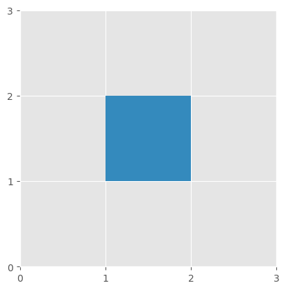
Rectangles are easily constructed.
rectangle \( R=\{a\le x\le b,c\le y\le d\} \)
Circles are not easily constructed. In fact, the equation of a circle in rectangular coordinates is not a function.
We would like a coordinate system suited to constructing circles, a “circular” coordinate system. Such a polar coordinate system in which circles are centered at the origin prioritizes circles over rectangles. In other words, circles are a more fundamental shape in a polar system.
Show code cell source
plt.style.use('ggplot');
fig, ax = plt.subplots()
ax.set_aspect(1);
ax.add_patch(mpl.patches.Rectangle((1,1),1,1));
ax.set_xticks(np.arange(0,4,1));
ax.set_xlim(0,3);
ax.set_yticks(np.arange(0,4,1));
ax.set_ylim(0,3);
Polar Coordinate System#
A point is described by \((r,\theta)\) where
\(r\) the distance of a point from the origin
\(\theta\) the angle of the point from the positive x-axis in the xy-plane.
The \(r\)-gridlines given by \(r=a\) are circles with constant radius from the origin and \(r=0\) is the origin.
The \(\theta\)-gridlines given by \(\theta=b\) are lines that go through the origin at a constant angle.
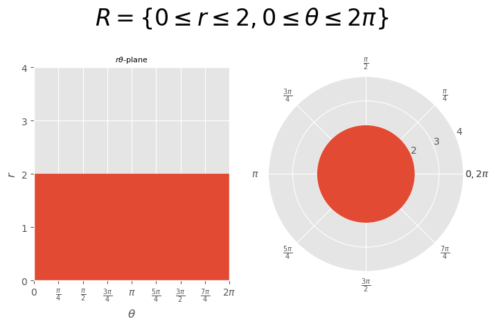
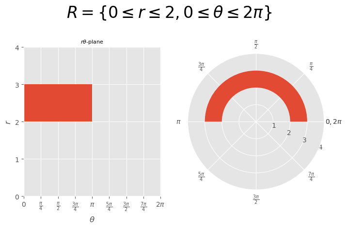
polar rectangles \( R=\{a\le r\le b,c\le\theta\le d\} \) form circles, sectors, and portions of these.
(1) It is usually desirable that \(r\ge0\), but not always. When \(r\lt0\), the curve is drawn in the opposite quadrant.
(2) It is usually desirable that \(0\le\theta\le2\pi\), but sometimes it is desirable that \(-\pi\le\theta\le\pi\).
Without restrictions (1) and (2), each point has multiple “addresses”. For example, the point \((0,2)\in\mathbb{R}^2\) has polar “addresses” \(\left(2,\frac{\pi}{2}\right),\left(2,\frac{5\pi}{2}\right),\left(-2,\frac{3\pi}{2}\right)\).
All points of the form \((0,\theta)\) lie at the origin since \(r=0\).
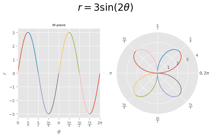
Graphing trigonometric functions in polar coordinates produces flower-like graphs called roses whose number of petals depends on the period of the function.
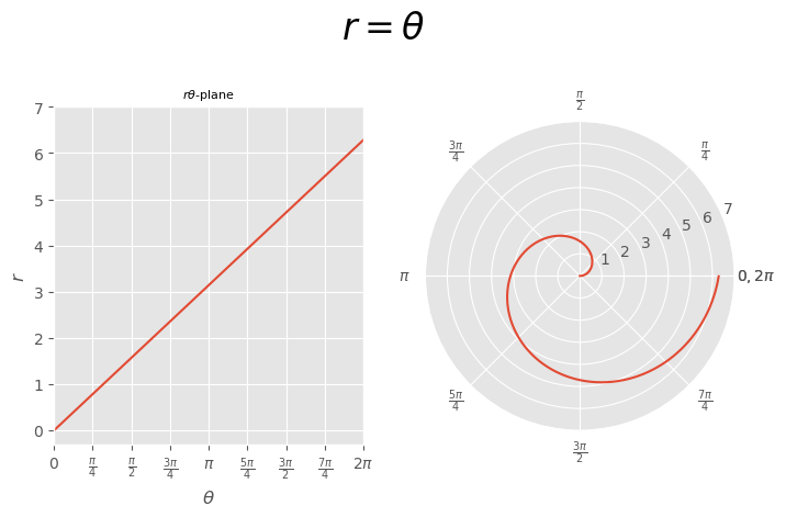
Linear functions in polar coordinates produce spirals.
Polar Transformation Equations#
\( \begin{aligned} x&=r\cos\theta\\ y&=r\sin\theta\\ x^2+y^2&=r^2\\ dA&=r\,dr\,d\theta\\ \end{aligned} \)
Easily converted to polar coordinates
circles centered at the origin (i.e., \(r\)-gridlines)
circles that intersect the origin
lines that go through the origin (i.e., \(\theta\)-gridlines)
vertical and horizontal lines
regions made up of these shapes
[EXAMPLE]
\( \begin{aligned} (r,\theta) &=\left(4,\frac{\pi}{3}\right)\\ \implies\\ (x,y) &=\left(4\cos\left(\frac{\pi}{3}\right),4\sin\left(\frac{\pi}{3}\right)\right) =(2,2\sqrt{3})\\ \end{aligned} \)
[EXAMPLE]
\( \begin{aligned} x^2+y^2=9 \implies r^2=9 \implies \sqrt{r^2}=\pm\sqrt{9} \implies r=\pm3 \implies r=3 \end{aligned} \)
[EXAMPLE]
\( \begin{aligned} y=x \implies r\sin\theta=r\cos\theta \implies \tan\theta=1 \implies \theta=\frac{\pi}{4} \end{aligned} \)
[EXAMPLE]
\( \begin{aligned} y=2 \implies r\sin\theta=2 \implies r=2\csc\theta \end{aligned} \)
[EXAMPLE]
\( \begin{aligned} (x-3)^2+y^2=9 \implies x^2-6x+9+y^2=9 \implies x^2+y^2=6x \implies r^2=6r\cos\theta \implies r=6\cos\theta \end{aligned} \)
[EXAMPLE]
\( \begin{aligned} f(x,y) =\frac{x+y^2}{\sqrt{x^2+y^2}} \implies f(r,\theta)=\frac{r\cos\theta+r^2\sin^2\theta}{\sqrt{r^2}} =\cos\theta+r\sin^2\theta \end{aligned} \)
\( \begin{aligned} f(2,2\sqrt{3}) =\frac{2+12}{\sqrt{4+12}} =\frac{14}{4} =\frac{7}{2} \end{aligned} \)
\( \begin{aligned} f\left(4,\frac{\pi}{3}\right) =\cos\left(\frac{\pi}{3}\right)+4\sin^2\left(\frac{\pi}{3}\right) =\frac{1}{2}+4\left(\frac{\sqrt{3}}{2}\right)^2 =\frac{1}{2}+3 =\frac{7}{2} \end{aligned} \)
Derivation of the last polar transformation equation via Jacobian#
There is another polar transformation equation besides
\( \begin{aligned} x&=r\cos\theta\\ y&=r\sin\theta\\ x^2+y^2&=r^2\\ \end{aligned} \)
which is important for integration which shows a fundamental difference between rectangular coordinates and polar coordinates.
All rectangular gridboxes have the same size.
\( dA=dx\,dy \)
Even though the range of gridboxes look the same in the \(r\theta\)-plane, they are actually different sizes in the polar plane: polar gridboxes do not have the same size everywhere even though they have the same \(dr\) and \(d\theta\).
\( dA\ne dr\,d\theta \)
The infinitesimal polar gridboxes can be approximated by parallelograms. This approximation becomes exact as \(dr,d\theta\rightarrow0\).
In \(\mathbb{R}^2\), we can use the \(2\times2\) determinant of first derivatives, called the Jacobian, to calculate the area of the rectangle.
\( \begin{aligned} x(r,\theta)&=r\cos\theta\\ y(r,\theta)&=r\sin\theta\\ \end{aligned} \rightarrow \begin{bmatrix} \frac{\partial x}{\partial r}&\frac{\partial x}{\partial\theta}\\ \frac{\partial y}{\partial r}&\frac{\partial y}{\partial\theta}\\ \end{bmatrix} =\begin{bmatrix} \cos\theta&-r\sin\theta\\ \sin\theta&r\cos\theta\\ \end{bmatrix} =r\cos^2\theta+r\sin^2\theta =r \)
\( dA=r\,dr\,d\theta \)
The Jacobian of the transformation keeps track of the size of gridboxes between rectangular coordinates and polar coordinates.
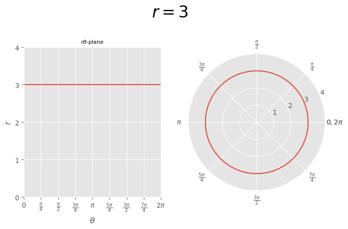
[Example] \(r=3\)#
[EXAMPLE]
\( r=3 \)
Show code cell source
theta = np.arange(0, 2 * np.pi, 0.01) # 0 ≤ θ ≤ 2π
r     = 3 + 0*theta                   # r = 3 constant

f   = 4
plt.style.use('ggplot');
fig = plt.figure(figsize=(2*f,f));

ax1 = plt.subplot(121, projection='rectilinear');
ax1.plot(theta,r);
ax1.set_xticks(ticks =np.arange(0,9*np.pi/4,np.pi/4),
               labels=[
                '$0$',
                '$\\frac{\\pi}{4}$',
                '$\\frac{\\pi}{2}$',
                '$\\frac{3\\pi}{4}$',
                '$\\pi$',
                '$\\frac{5\\pi}{4}$',
                '$\\frac{3\\pi}{2}$',
                '$\\frac{7\\pi}{4}$',
                '$2\\pi$'
               ]);
ax1.set_xlim(0,2*np.pi);
ax1.set_xlabel('$\\theta$');
ax1.set_yticks(ticks =np.arange(0,5,1));
ax1.set_ylabel('$r$');
ax1.set_title('$r\\theta$-plane', fontsize=8);
ax1.grid(True);

ax2 = plt.subplot(122, projection='polar');
ax2.plot(theta, r);
ax2.set_rticks(ticks =np.arange(0,8,1),
               labels=['','1','2','3','4','5','6','7']);
ax2.set_xticks(ticks =np.arange(0,9*np.pi/4,np.pi/4),
               labels=[
                '$0,2\\pi$',
                '$\\frac{\\pi}{4}$',
                '$\\frac{\\pi}{2}$',
                '$\\frac{3\\pi}{4}$',
                '$\\pi$',
                '$\\frac{5\\pi}{4}$',
                '$\\frac{3\\pi}{2}$',
                '$\\frac{7\\pi}{4}$',
                '$0,2\\pi$'
               ]);
ax2.set_rmax(4);
ax2.grid(True);

fig.suptitle('$r=3$', fontsize=24, y=1.1);
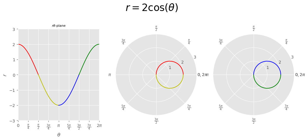
[Example] \(r=2\cos\theta\)#
[EXAMPLE]
\( r=2\cos\theta \)
Show code cell source
theta1 = np.arange(0, np.pi/2, 0.01)
r1     = 2 * np.cos(theta1)
theta2 = np.arange(np.pi/2, np.pi, 0.01)
r2     = 2 * np.cos(theta2)
theta3 = np.arange(np.pi, 3*np.pi/2, 0.01)
r3     = 2 * np.cos(theta3)
theta4 = np.arange(3*np.pi/2, 2*np.pi, 0.01)
r4     = 2 * np.cos(theta4)

f   = 4
plt.style.use('ggplot');
fig = plt.figure(figsize=(3*f,f));

ax1 = plt.subplot(131, projection='rectilinear');
ax1.plot(theta1,r1,color='r');
ax1.plot(theta2,r2,color='y');
ax1.plot(theta3,r3,color='b');
ax1.plot(theta4,r4,color='g');
ax1.set_xticks(ticks =np.arange(0,9*np.pi/4,np.pi/4),
               labels=[
                '$0$',
                '$\\frac{\\pi}{4}$',
                '$\\frac{\\pi}{2}$',
                '$\\frac{3\\pi}{4}$',
                '$\\pi$',
                '$\\frac{5\\pi}{4}$',
                '$\\frac{3\\pi}{2}$',
                '$\\frac{7\\pi}{4}$',
                '$2\\pi$'
               ]);
ax1.set_xlim(0,2*np.pi);
ax1.set_xlabel('$\\theta$');
ax1.set_yticks(ticks =np.arange(-3,4,1));
ax1.set_ylabel('$r$');
ax1.set_title('$r\\theta$-plane', fontsize=8);
ax1.grid(True);

ax2 = plt.subplot(132, projection='polar');
ax2.plot(theta1, r1, color='r');
ax2.plot(theta2+np.pi, np.abs(r2),color='y');
ax2.set_rticks(ticks =np.arange(0,5,1),
               labels=['','1','2','3','4']);
ax2.set_xticks(ticks =np.arange(0,9*np.pi/4,np.pi/4),
               labels=[
                '$0,2\\pi$',
                '$\\frac{\\pi}{4}$',
                '$\\frac{\\pi}{2}$',
                '$\\frac{3\\pi}{4}$',
                '$\\pi$',
                '$\\frac{5\\pi}{4}$',
                '$\\frac{3\\pi}{2}$',
                '$\\frac{7\\pi}{4}$',
                '$0,2\\pi$'
               ]);
ax2.set_rmax(3);
ax2.grid(True);

ax3 = plt.subplot(133, projection='polar');
ax3.plot(theta3+np.pi, np.abs(r3),color='b');
ax3.plot(theta4, r4, color='g');
ax3.set_rticks(ticks =np.arange(0,5,1),
               labels=['','1','2','3','4']);
ax3.set_xticks(ticks =np.arange(0,9*np.pi/4,np.pi/4),
               labels=[
                '$0,2\\pi$',
                '$\\frac{\\pi}{4}$',
                '$\\frac{\\pi}{2}$',
                '$\\frac{3\\pi}{4}$',
                '$\\pi$',
                '$\\frac{5\\pi}{4}$',
                '$\\frac{3\\pi}{2}$',
                '$\\frac{7\\pi}{4}$',
                '$0,2\\pi$'
               ]);
ax3.set_rmax(3);
ax3.grid(True);

fig.suptitle('$r=2\\cos(\\theta)$', fontsize=24, y=1.1);
[Example] \(r=3\sin(2\theta)\)#
[EXAMPLE]
\( r=3\sin(2\theta) \)
Show code cell source
theta1 = np.arange((0/4)*np.pi, (1/4)*np.pi, 0.01)
r1     = 3 * np.sin(2*theta1)
theta2 = np.arange((1/4)*np.pi, (2/4)*np.pi, 0.01)
r2     = 3 * np.sin(2*theta2)
theta3 = np.arange((2/4)*np.pi, (3/4)*np.pi, 0.01)
r3     = 3 * np.sin(2*theta3)
theta4 = np.arange((3/4)*np.pi, (4/4)*np.pi, 0.01)
r4     = 3 * np.sin(2*theta4)
theta5 = np.arange((4/4)*np.pi, (5/4)*np.pi, 0.01)
r5     = 3 * np.sin(2*theta5)
theta6 = np.arange((5/4)*np.pi, (6/4)*np.pi, 0.01)
r6     = 3 * np.sin(2*theta6)
theta7 = np.arange((6/4)*np.pi, (7/4)*np.pi, 0.01)
r7     = 3 * np.sin(2*theta7)
theta8 = np.arange((7/4)*np.pi, (8/4)*np.pi, 0.01)
r8     = 3 * np.sin(2*theta8)

f   = 4
plt.style.use('ggplot');
fig = plt.figure(figsize=(2*f,f));

ax1 = plt.subplot(121, projection='rectilinear');
ax1.plot(theta1,r1);
ax1.plot(theta2,r2);
ax1.plot(theta3,r3);
ax1.plot(theta4,r4);
ax1.plot(theta5,r5);
ax1.plot(theta6,r6);
ax1.plot(theta7,r7);
ax1.plot(theta8,r8);
ax1.set_xticks(ticks =np.arange(0,9*np.pi/4,np.pi/4),
               labels=[
                '$0$',
                '$\\frac{\\pi}{4}$',
                '$\\frac{\\pi}{2}$',
                '$\\frac{3\\pi}{4}$',
                '$\\pi$',
                '$\\frac{5\\pi}{4}$',
                '$\\frac{3\\pi}{2}$',
                '$\\frac{7\\pi}{4}$',
                '$2\\pi$'
               ]);
ax1.set_xlim(0,2*np.pi);
ax1.set_xlabel('$\\theta$');
ax1.set_yticks(ticks =np.arange(-3,4,1));
ax1.set_ylabel('$r$');
ax1.set_title('$r\\theta$-plane', fontsize=8);
ax1.grid(True);

ax2 = plt.subplot(122, projection='polar');
ax2.plot(theta1,r1);
ax2.plot(theta2,r2);
ax2.plot(theta3+np.pi,np.abs(r3));
ax2.plot(theta4+np.pi,np.abs(r4));
ax2.plot(theta5,r5);
ax2.plot(theta6,r6);
ax2.plot(theta7+np.pi,np.abs(r7));
ax2.plot(theta8+np.pi,np.abs(r8));
ax2.set_rticks(ticks =np.arange(0,5,1),
               labels=['','1','2','3','4']);
ax2.set_xticks(ticks =np.arange(0,9*np.pi/4,np.pi/4),
               labels=[
                '$0,2\\pi$',
                '$\\frac{\\pi}{4}$',
                '$\\frac{\\pi}{2}$',
                '$\\frac{3\\pi}{4}$',
                '$\\pi$',
                '$\\frac{5\\pi}{4}$',
                '$\\frac{3\\pi}{2}$',
                '$\\frac{7\\pi}{4}$',
                '$0,2\\pi$'
               ]);
ax2.set_rmax(4);
ax2.grid(True);

fig.suptitle('$r=3\\sin(2\\theta)$', fontsize=24, y=1.1);
[Example] \(r=\theta\)#
[EXAMPLE]
\( r=\theta \)
Show code cell source
theta = np.arange(0, 2 * np.pi, 0.01) # 0 ≤ θ ≤ 2π
r     = theta                         # r = θ

f   = 4
plt.style.use('ggplot');
fig = plt.figure(figsize=(2*f,f));

ax1 = plt.subplot(121, projection='rectilinear');
ax1.plot(theta,r);
ax1.set_xticks(ticks =np.arange(0,9*np.pi/4,np.pi/4),
               labels=[
                '$0$',
                '$\\frac{\\pi}{4}$',
                '$\\frac{\\pi}{2}$',
                '$\\frac{3\\pi}{4}$',
                '$\\pi$',
                '$\\frac{5\\pi}{4}$',
                '$\\frac{3\\pi}{2}$',
                '$\\frac{7\\pi}{4}$',
                '$2\\pi$'
               ]);
ax1.set_xlim(0,2*np.pi);
ax1.set_xlabel('$\\theta$');
ax1.set_yticks(ticks =np.arange(0,8,1));
ax1.set_ylabel('$r$');
ax1.set_title('$r\\theta$-plane', fontsize=8);
ax1.grid(True);

ax2 = plt.subplot(122, projection='polar');
ax2.plot(theta, r);
ax2.set_rticks(ticks =np.arange(0,8,1),
               labels=['','1','2','3','4','5','6','7']);
ax2.set_xticks(ticks =np.arange(0,9*np.pi/4,np.pi/4),
               labels=[
                '$0,2\\pi$',
                '$\\frac{\\pi}{4}$',
                '$\\frac{\\pi}{2}$',
                '$\\frac{3\\pi}{4}$',
                '$\\pi$',
                '$\\frac{5\\pi}{4}$',
                '$\\frac{3\\pi}{2}$',
                '$\\frac{7\\pi}{4}$',
                '$0,2\\pi$'
               ]);
ax2.set_rmax(7);
ax2.grid(True);
#ax2.set_rlabel_position();

fig.suptitle('$r=\\theta$', fontsize=24, y=1.1);
[Example] \(R=\{0\le r\le2,0\le\theta\le2\pi\}\)#
\( R=\{0\le r\le2,0\le\theta\le2\pi\} \)
Show code cell source
r1 = 0
r2 = 2
t1 = 0
t2 = 2*np.pi

f   = 4
plt.style.use('ggplot');
fig = plt.figure(figsize=(2*f,f));

ax1 = plt.subplot(121, projection='rectilinear');
ax1.bar(x=t2-(t2-t1)/2,height=r2-r1,width=t2-t1,bottom=r1);
ax1.set_xticks(ticks =np.arange(0,9*np.pi/4,np.pi/4),
               labels=[
                '$0$',
                '$\\frac{\\pi}{4}$',
                '$\\frac{\\pi}{2}$',
                '$\\frac{3\\pi}{4}$',
                '$\\pi$',
                '$\\frac{5\\pi}{4}$',
                '$\\frac{3\\pi}{2}$',
                '$\\frac{7\\pi}{4}$',
                '$2\\pi$'
               ]);
ax1.set_xlim(0,2*np.pi);
ax1.set_xlabel('$\\theta$');
ax1.set_yticks(ticks =np.arange(0,8,1));
ax1.set_ylim(0,4);
ax1.set_ylabel('$r$');
ax1.set_title('$r\\theta$-plane', fontsize=8);
ax1.grid(True);

ax2 = plt.subplot(122, projection='polar');
ax2.bar(x=t2-(t2-t1)/2,height=r2-r1,width=t2-t1,bottom=r1);
ax2.set_rticks(ticks =np.arange(0,8,1),
               labels=['','1','2','3','4','5','6','7']);
ax2.set_xticks(ticks =np.arange(0,9*np.pi/4,np.pi/4),
               labels=[
                '$0,2\\pi$',
                '$\\frac{\\pi}{4}$',
                '$\\frac{\\pi}{2}$',
                '$\\frac{3\\pi}{4}$',
                '$\\pi$',
                '$\\frac{5\\pi}{4}$',
                '$\\frac{3\\pi}{2}$',
                '$\\frac{7\\pi}{4}$',
                '$0,2\\pi$'
               ]);
ax2.set_rmax(4);
ax2.grid(True);
#ax2.set_rlabel_position();

fig.suptitle('$R=\\{0\\leq r\\leq2,0\\leq\\theta\\leq2\\pi\\}$', fontsize=24, y=1.1);
[Example] \(R=\{2\le r\le3,0\le\theta\le\pi\}\)#
\( R=\{2\le r\le3,0\le\theta\le\pi\} \)
Show code cell source
r1 = 2
r2 = 3
t1 = 0
t2 = np.pi

f   = 4
plt.style.use('ggplot');
fig = plt.figure(figsize=(2*f,f));

ax1 = plt.subplot(121, projection='rectilinear');
ax1.bar(x=t2-(t2-t1)/2,height=r2-r1,width=t2-t1,bottom=r1);
ax1.set_xticks(ticks =np.arange(0,9*np.pi/4,np.pi/4),
               labels=[
                '$0$',
                '$\\frac{\\pi}{4}$',
                '$\\frac{\\pi}{2}$',
                '$\\frac{3\\pi}{4}$',
                '$\\pi$',
                '$\\frac{5\\pi}{4}$',
                '$\\frac{3\\pi}{2}$',
                '$\\frac{7\\pi}{4}$',
                '$2\\pi$'
               ]);
ax1.set_xlim(0,2*np.pi);
ax1.set_xlabel('$\\theta$');
ax1.set_yticks(ticks =np.arange(0,8,1));
ax1.set_ylim(0,4);
ax1.set_ylabel('$r$');
ax1.set_title('$r\\theta$-plane', fontsize=8);
ax1.grid(True);

ax2 = plt.subplot(122, projection='polar');
ax2.bar(x=t2-(t2-t1)/2,height=r2-r1,width=t2-t1,bottom=r1);
ax2.set_rticks(ticks =np.arange(0,8,1),
               labels=['','1','2','3','4','5','6','7']);
ax2.set_xticks(ticks =np.arange(0,9*np.pi/4,np.pi/4),
               labels=[
                '$0,2\\pi$',
                '$\\frac{\\pi}{4}$',
                '$\\frac{\\pi}{2}$',
                '$\\frac{3\\pi}{4}$',
                '$\\pi$',
                '$\\frac{5\\pi}{4}$',
                '$\\frac{3\\pi}{2}$',
                '$\\frac{7\\pi}{4}$',
                '$0,2\\pi$'
               ]);
ax2.set_rmax(4);
ax2.grid(True);
ax2.set_rlabel_position(-25);

fig.suptitle('$R=\\{0\\leq r\\leq2,0\\leq\\theta\\leq2\\pi\\}$', fontsize=24, y=1.1);
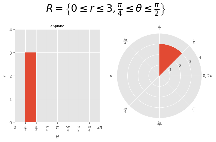
[Example] \(\begin{aligned}R=\left\{0\le r\le3,\frac{\pi}{4}\le\theta\le\frac{\pi}{2}\right\}\end{aligned}\)#
\( \begin{aligned} R=\left\{0\le r\le3,\frac{\pi}{4}\le\theta\le\frac{\pi}{2}\right\} \end{aligned} \)
Show code cell source
r1 = 0
r2 = 3
t1 = np.pi/4
t2 = np.pi/2

f   = 4
plt.style.use('ggplot');
fig = plt.figure(figsize=(2*f,f));

ax1 = plt.subplot(121, projection='rectilinear');
ax1.bar(x=t2-(t2-t1)/2,height=r2-r1,width=t2-t1,bottom=r1);
ax1.set_xticks(ticks =np.arange(0,9*np.pi/4,np.pi/4),
               labels=[
                '$0$',
                '$\\frac{\\pi}{4}$',
                '$\\frac{\\pi}{2}$',
                '$\\frac{3\\pi}{4}$',
                '$\\pi$',
                '$\\frac{5\\pi}{4}$',
                '$\\frac{3\\pi}{2}$',
                '$\\frac{7\\pi}{4}$',
                '$2\\pi$'
               ]);
ax1.set_xlim(0,2*np.pi);
ax1.set_xlabel('$\\theta$');
ax1.set_yticks(ticks =np.arange(0,8,1));
ax1.set_ylim(0,4);
ax1.set_ylabel('$r$');
ax1.set_title('$r\\theta$-plane', fontsize=8);
ax1.grid(True);

ax2 = plt.subplot(122, projection='polar');
ax2.bar(x=t2-(t2-t1)/2,height=r2-r1,width=t2-t1,bottom=r1);
ax2.set_rticks(ticks =np.arange(0,8,1),
               labels=['','1','2','3','4','5','6','7']);
ax2.set_xticks(ticks =np.arange(0,9*np.pi/4,np.pi/4),
               labels=[
                '$0,2\\pi$',
                '$\\frac{\\pi}{4}$',
                '$\\frac{\\pi}{2}$',
                '$\\frac{3\\pi}{4}$',
                '$\\pi$',
                '$\\frac{5\\pi}{4}$',
                '$\\frac{3\\pi}{2}$',
                '$\\frac{7\\pi}{4}$',
                '$0,2\\pi$'
               ]);
ax2.set_rmax(4);
ax2.grid(True);
#ax2.set_rlabel_position();

fig.suptitle('$R=\\left\\{0\\leq r\\leq3,\\frac{\\pi}{4}\\leq\\theta\\leq\\frac{\\pi}{2}\\right\\}$', fontsize=24, y=1.1);
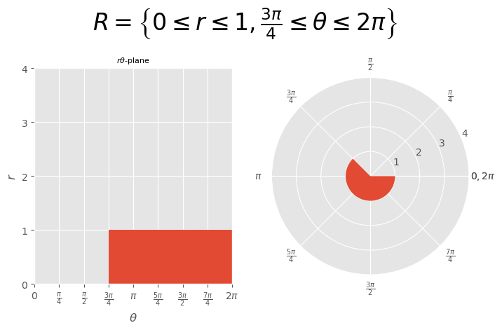
[Example] \(\begin{aligned}R=\left\{0\le r\le1,\frac{3\pi}{4}\le\theta\le2\pi\right\}\end{aligned}\)#
\( \begin{aligned} R=\left\{0\le r\le1,\frac{3\pi}{4}\le\theta\le2\pi\right\} \end{aligned} \)
Show code cell source
r1 = 0
r2 = 1
t1 = 3*np.pi/4
t2 = 2*np.pi

f   = 4
plt.style.use('ggplot');
fig = plt.figure(figsize=(2*f,f));

ax1 = plt.subplot(121, projection='rectilinear');
ax1.bar(x=t2-(t2-t1)/2,height=r2-r1,width=t2-t1,bottom=r1);
ax1.set_xticks(ticks =np.arange(0,9*np.pi/4,np.pi/4),
               labels=[
                '$0$',
                '$\\frac{\\pi}{4}$',
                '$\\frac{\\pi}{2}$',
                '$\\frac{3\\pi}{4}$',
                '$\\pi$',
                '$\\frac{5\\pi}{4}$',
                '$\\frac{3\\pi}{2}$',
                '$\\frac{7\\pi}{4}$',
                '$2\\pi$'
               ]);
ax1.set_xlim(0,2*np.pi);
ax1.set_xlabel('$\\theta$');
ax1.set_yticks(ticks =np.arange(0,8,1));
ax1.set_ylim(0,4);
ax1.set_ylabel('$r$');
ax1.set_title('$r\\theta$-plane', fontsize=8);
ax1.grid(True);

ax2 = plt.subplot(122, projection='polar');
ax2.bar(x=t2-(t2-t1)/2,height=r2-r1,width=t2-t1,bottom=r1);
ax2.set_rticks(ticks =np.arange(0,8,1),
               labels=['','1','2','3','4','5','6','7']);
ax2.set_xticks(ticks =np.arange(0,9*np.pi/4,np.pi/4),
               labels=[
                '$0,2\\pi$',
                '$\\frac{\\pi}{4}$',
                '$\\frac{\\pi}{2}$',
                '$\\frac{3\\pi}{4}$',
                '$\\pi$',
                '$\\frac{5\\pi}{4}$',
                '$\\frac{3\\pi}{2}$',
                '$\\frac{7\\pi}{4}$',
                '$0,2\\pi$'
               ]);
ax2.set_rmax(4);
ax2.grid(True);
#ax2.set_rlabel_position();

fig.suptitle('$R=\\left\\{0\\leq r\\leq1,\\frac{3\\pi}{4}\\leq\\theta\\leq2\\pi\\right\\}$', fontsize=24, y=1.1);